Introduction to Psychometrics

Psychometric and Statistical Primer

Welcome!

Introduction

Some things about me:

• Graduated from this program in 2015 (Triple Dawg!)
• Currently a manager on McKinsey & Company’s internal People, Analytics, & Measurement (PAM) team
• Love all things analytics!

Your turn!

Round Robin!

• What’s your name?
• What are you studying?
• Do you hate, tolerate, or love methods courses?

What We’ll Cover

Course Goals

• Psychometric Theories & Survey Development
  • Classical Test Theory, Generalizability Theory, & Validity Theory
• Statistical Modeling
  • Latent Variable Models, Network Models
• R Programming

Goals of this Lecture

• Overview of Psychometrics
  • The Theoretical: Test Theories & Latent Variable Models
  • The Practical: Assessment / Questionnaire Design
• Statistical Primer
  • Review of Probability Theory
  • Review of Statistical Inference

What is Psychometics?

Psychometrics, or quantitative psychology, is the disciplinary home of a set of statistical models and methods that have been developed primarily to summarize, describe, and draw inferences from empirical data collected in psychological research.

Jones & Thissen, 2007

The Theoretical Side

Theory & Methods in Psychometrics

• Test Theory: A mixture of theoretical and statistical models that have been developed to advance educational and psychological measurement.

• Latent Variable Models: A family of statistical models that explain statistical dependencies among sets of observed random variables (e.g. survey responses) by appealing to variation in a smaller set of unobserved (latent) variables.

Test Theories in Psychometrics

• There are three major test theories in Psychometrics:

  • Classical Test Theory (CTT)
  • Generalizability Theory (GT)
  • Item Response Theory (IRT)

• The above theories have introduced and further refined the theories of test validity and test reliability.

Classical Test Theory

• CTT set the foundations for future test theories with the idea that an individual’s observed test score is composed of two different additive components: True Score and Error.

• Through its introduction of True Score and Error, CTT helped to formalize the theories of test validity and reliability.

\[\text{Observed Score} = \text{True Score} + \text{Error}\]

Generalizability Theory

• Built on CTT by further specifying the different sources of error that comprise an individual’s observed score.

• GT really furthered the development of reliability theory by introducing different types of reliability indices and drawing a distinction between relative and absolute test score comparisons.

\[\text{Observed Scored} = \mu + E_{rater} + E_{item} + E_{rater\times{}item}\]

Item Response Theory

• IRT is a modern measurement theory that focuses on the measurement characteristics of the individual items that make up an assessment.

• Unlike CTT and GT, IRT estimates measurement characteristics of the individual items independently from the abilities of the test takers—this is a big plus!

\[p(x_{ij} = 1 |\theta_{i},b_{j},a_{j})=\frac{1}{1 + e^{-a_{j}(\theta_{i}-b_{j})}}\]

Latent Variable Models: An Overview

• A family of statistical models that relate covariation in observable variables (e.g. item responses) to latent variables (e.g. psychological constructs).

• Essentially allows one to use observed measurements to infer something about an unobservable construct.

	Manifest Variable Distribution
Latent Variable Distribution	Continuous	Categorical
Continuous	Factor Analysis	Item Response Theory
Categorical	Latent Profile Analysis	Latent Class Analysis

The Practical Side

Some Survey Jargon

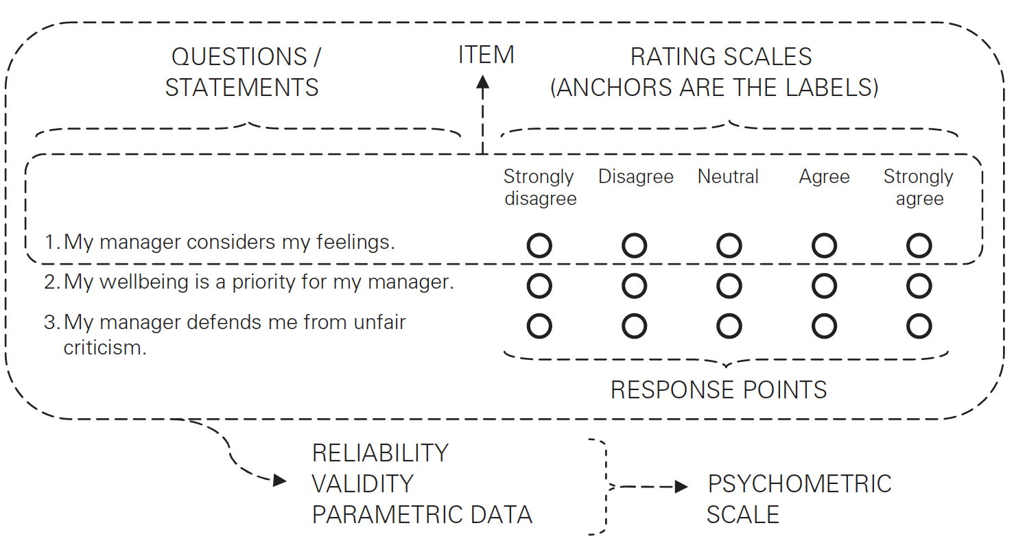
Robinson (2018). Using multi-item psychometric scales for research and practice in human resource management

The Many Uses of Surveys and Assessments

• Surveys / Assessments are used to assess a wide variety of constructs:
  • Educational Assessment (SAT, GRE)
  • Mental health disorders (Beck’s Depression Inventory)
  • Personality (Hogan PEI, Big 5 scales)
  • Employee Attitude Surveys (There are many!)
  • Employee Knowledge, Skills, Abilities (KSAs!)

The Scale Development Process

• Developing the Scale
  • Build a measurement framework
  • Generate items
  • Evaluate preliminary items
• Testing the Scale
  • Pilot the new scale
  • Analyze the pilot data
  • Repeat if needed & possible
• Put the scale into operation

Probability Theory and Statistical Inference

A Reassuring Reminder

Statistics is hard, especially when effects are small and variable and measurements are noisy.

McShane et al., 2019

Who cares?

• Why do we care about probability theory and statistical inference? What have they ever done for us?

Statistical Inference

• Statistical inference is about drawing conclusions about an entire population based on the information in a sample.

Sterba, S. K. (2009). Alternative Model-Based and Design-Based Frameworks for Inference From Samples to Populations

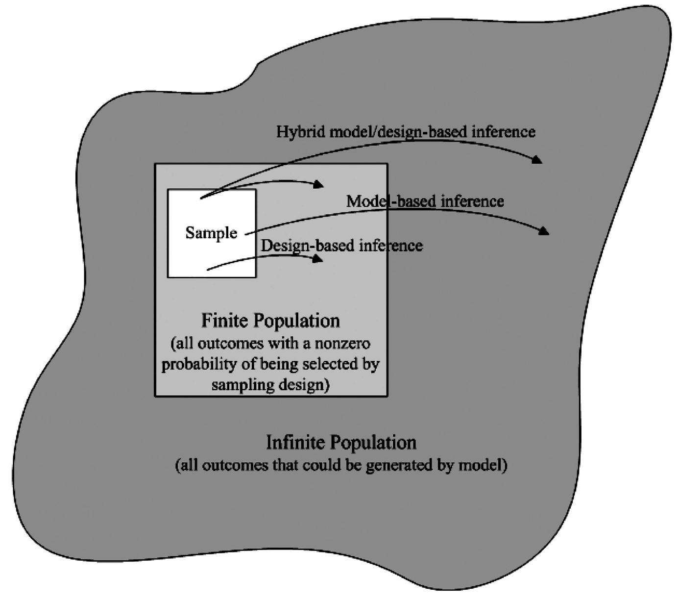
Model-Based Statistical Inference

• Model-based inference allows us to make inferences to an infinite population from non-random samples as long as we are willing to make three (strong) assumptions:
  • Assume a generative statistical model
  • Assume parametric distributional assumptions on our model
  • Assume a selection mechanism

Model-Based Statistical Inference

\[\underbrace{y_{i}=\beta_{0} + \beta_{1}x_{i} + \epsilon_{i}}_{\text{Generative Model}}\]

\[\underbrace{\epsilon_{i}\stackrel{iid}{\sim}N(0, \sigma^{2})}_{\text{Parametric Assumptions & Selection Mech.}}\]

Role of Probability Theory in Statistics

\[y_{i}=\beta_{0} + \beta_{1}x_{i} + \epsilon_{i}\]

\[\to\]

\[\underbrace{f_{Y|X}(y_{i}|x_{i})}_{\text{Conditional}\\ \;\;\;\;\text{PDF}}\overbrace{\stackrel{iid}{\sim}}^{\;\;\text{Dist.}\\\text{Assump.}}\underbrace{N(\beta_{0} + \beta_{1}x_{i}, \sigma^{2})}_{\text{Normal PDF}}\]

What is Probability Theory?

• Probability theory is a mathematical construct used to represent processes involving randomness, unpredictability, or intrinsic uncertainty.

• Probability theory is a model! It allows for us to deal with the uncertainty that comes from being unable to measure every little thing that may be related to our outcome.

Philsophy of Probability and Inference

	Philosophy of Probability
Statistical Inference	Frequentist	Bayesian
Model Based	✖
Design Based

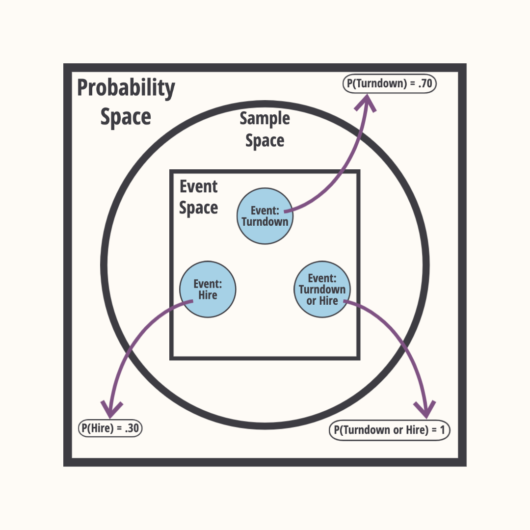
Random Generative Process (RGP)

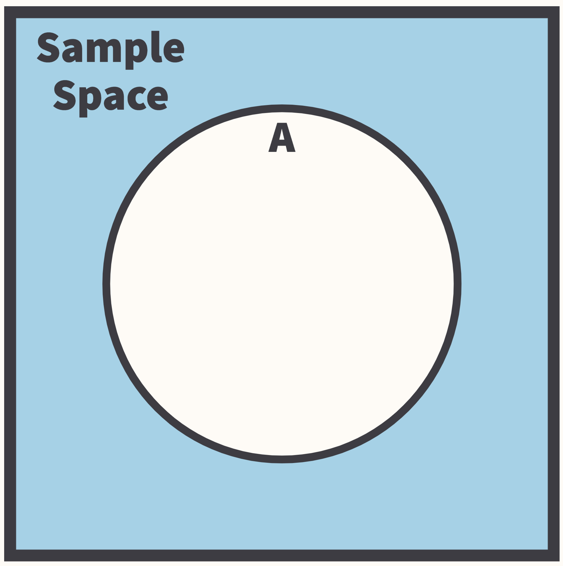
• Random Generative Process is a mechanism that selects an outcome from a set of multiple outcomes. It consists of three components:
  • Sample Space: Set of all possible states of an RGP.
  • Event Space: Subset of the sample space that consists of possible events that could occur across multiple states.
  • Probability Measure: A function that maps the event to a real number.

Probability Space: Properties

\(P(A \cup B) = P(A) + P(B)\)

\(B \subseteq A, P(B) \leq P(A)\)

\(P(A \cup B) = P(A) + P(B) - P(A \cap B)\)

\(P(A^{C}) = 1 - P(A)\)

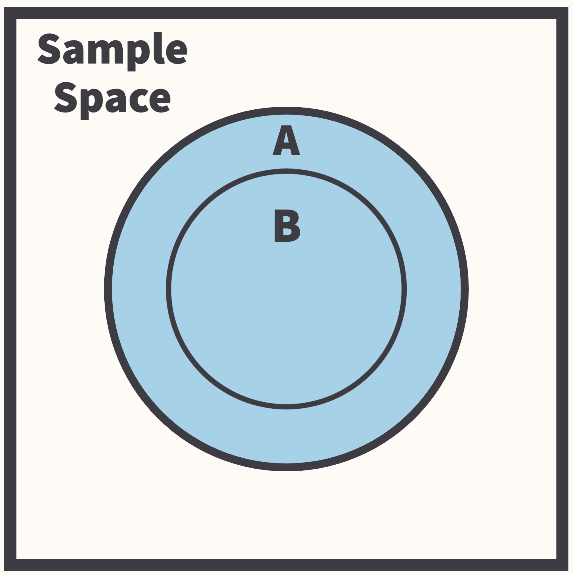
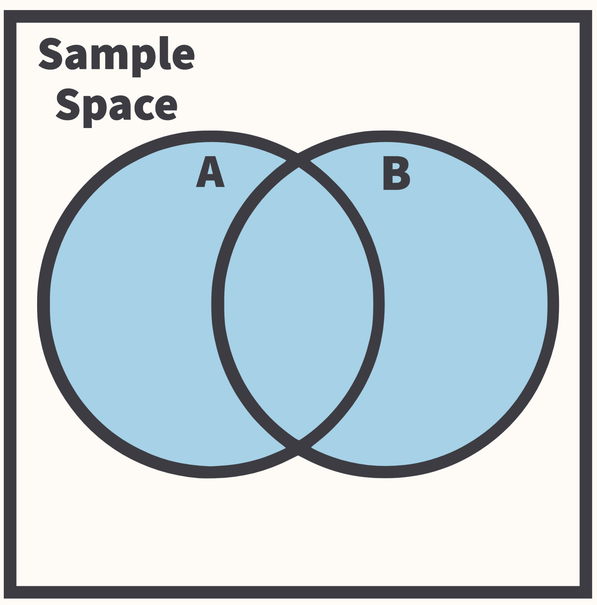
Joint & Conditional Probability

• Joint and conditional probability describe how the probabilities of two different events are related.

• Joint probability tells us the probability that two events will both occur:

  • \(P(A \cap B)\)

• Conditional probability tell us how the probability of one event changes given that another event already occurred:

  • \(P(A|B) = \frac{P(A \cap B)}{P(B)}\)

Employee Selection Example

For the next few slides, we will imagine we are an workforce analytics analyst on the recruiting team. We want to look at the relationship between a candidate’s select assessment performance, Assessment Outcome, and the organization’s selection decision, Hiring Outcome.

Joint Probabilities: Employee Selection

• The table displays the joint probabilities for Hiring Outcome and Assessment Outcome.
  • What is the probability that Hiring Outcome = Hire and Assessment Outcome = Fail?
  • What is the probability that Hiring Outcome = Hire and Assessment Outcome = Pass?

	Hire	Turndown
Fail	0.033	0.149
Pass	0.436	0.291
Pass+	0.071	0.020

Conditonal Probabilities

• The tables to the right display the conditional probabilities for Hiring Outcome and Assessment Outcome.
  • What is the probability that Hiring Outcome = Hire given that Assessment Outcome = Fail?
  • What is the probability that Assessment Outcome = Fail given that Hiring Category = Hire?

P(Selection Decision) given Assessment Outcome

	Hire	Turndown
Fail	0.182	0.818
Pass	0.600	0.400
Pass+	0.778	0.222

P(Assessment Outcome) given Selection Decision

	Hire	Turndown
Fail	0.061	0.323
Pass	0.808	0.633
Pass+	0.131	0.044

More Conditional Probabilities

• Multiplicative Law of Probability

\(P(A \cap B)=P(A|B)P(B)\)

• Independence

\(P(A \cap B) = P(A)P(B)\)

\(\begin{equation}\begin{aligned} P(A|B) &= \frac{P(A)P(B)}{P(B)} \\ &= P(A) \end{aligned}\end{equation}\)

• Bayes’ Rule

\(P(B|A) = \frac{P(A|B)P(B)}{P(A)}\)

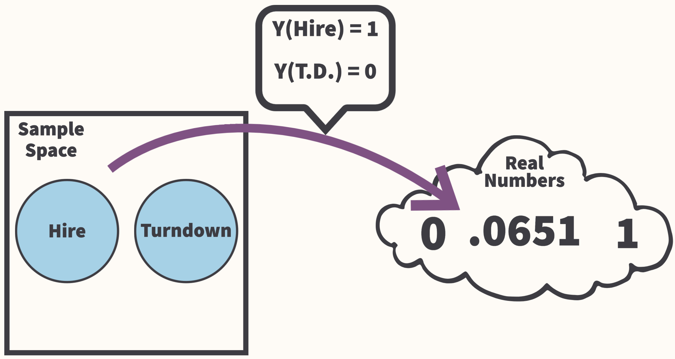
Random Variables

• Random variables are functions that take an event (Hire or Fire) as the input and output a real number (0 or 1).
• Random variables can be categorized as discrete or continuous based on the range of their output.
  • Discrete Variables have a countable infinite range (e.g. integer valued output)
  • Continuous Variables have an uncountable infinite range (e.g. real numbers)

Probability Functions

We can summarize the probabilities of random variables using two related probability functions: the Probability Mass (Density) Function and the Cumulative Distribution Function.

Discrete Variables

• Probability Mass Function (PMF):
  • \(f(x)=P(X=x)\)
• Cumulative Distribution Function (CDF)
  • \(F(x)=P(X \leq x)\)

Continuous Variables

• Probability Density Function (PDF):
  • \(f(x)=\frac{dF(u)}{du}|_{u=x}\)
• Cumulative Distribution Function (CDF):
  • \(F(x)=P(X \leq x) = \int_{-\infty}^{x}f(u)du\)

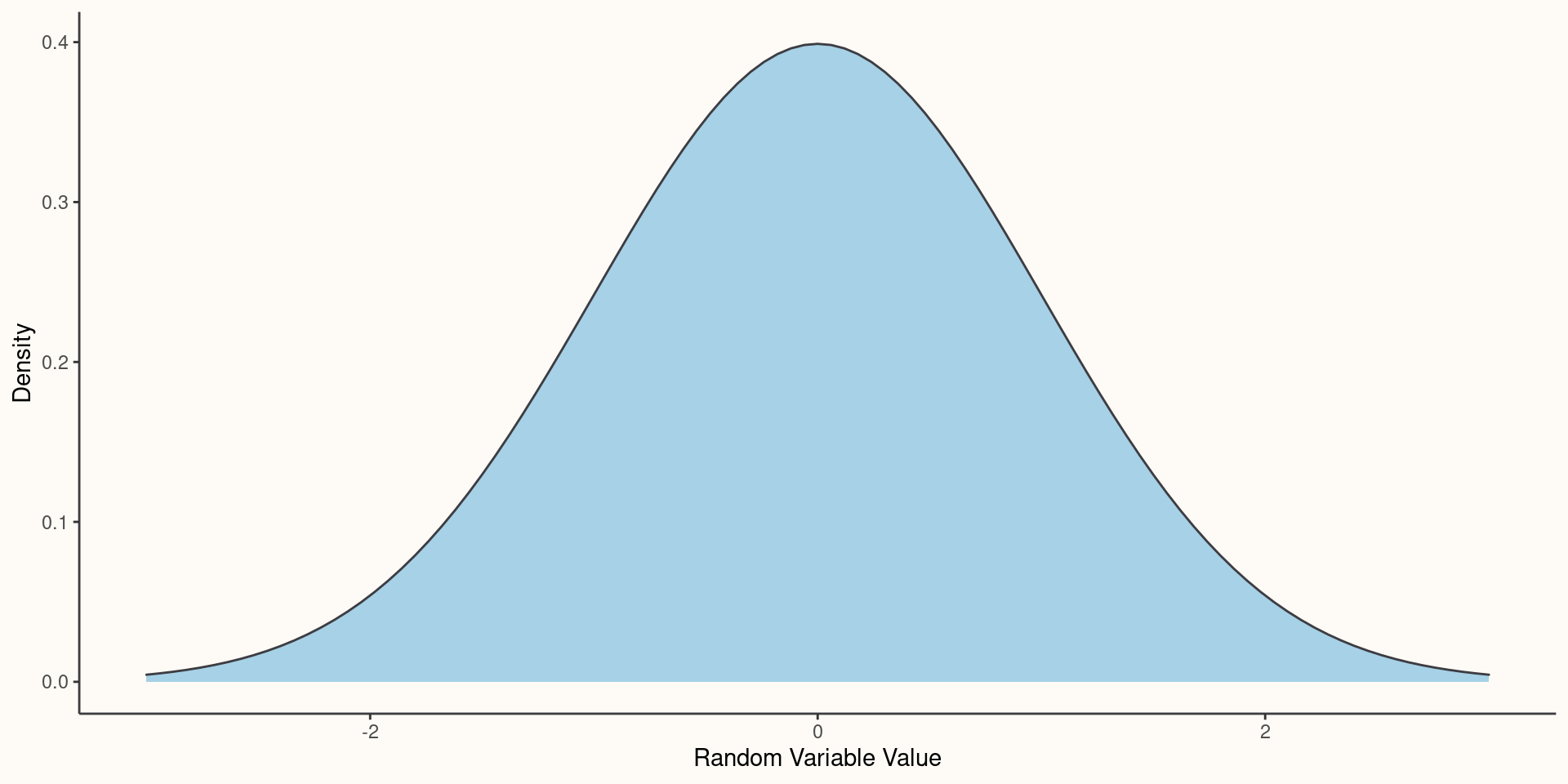
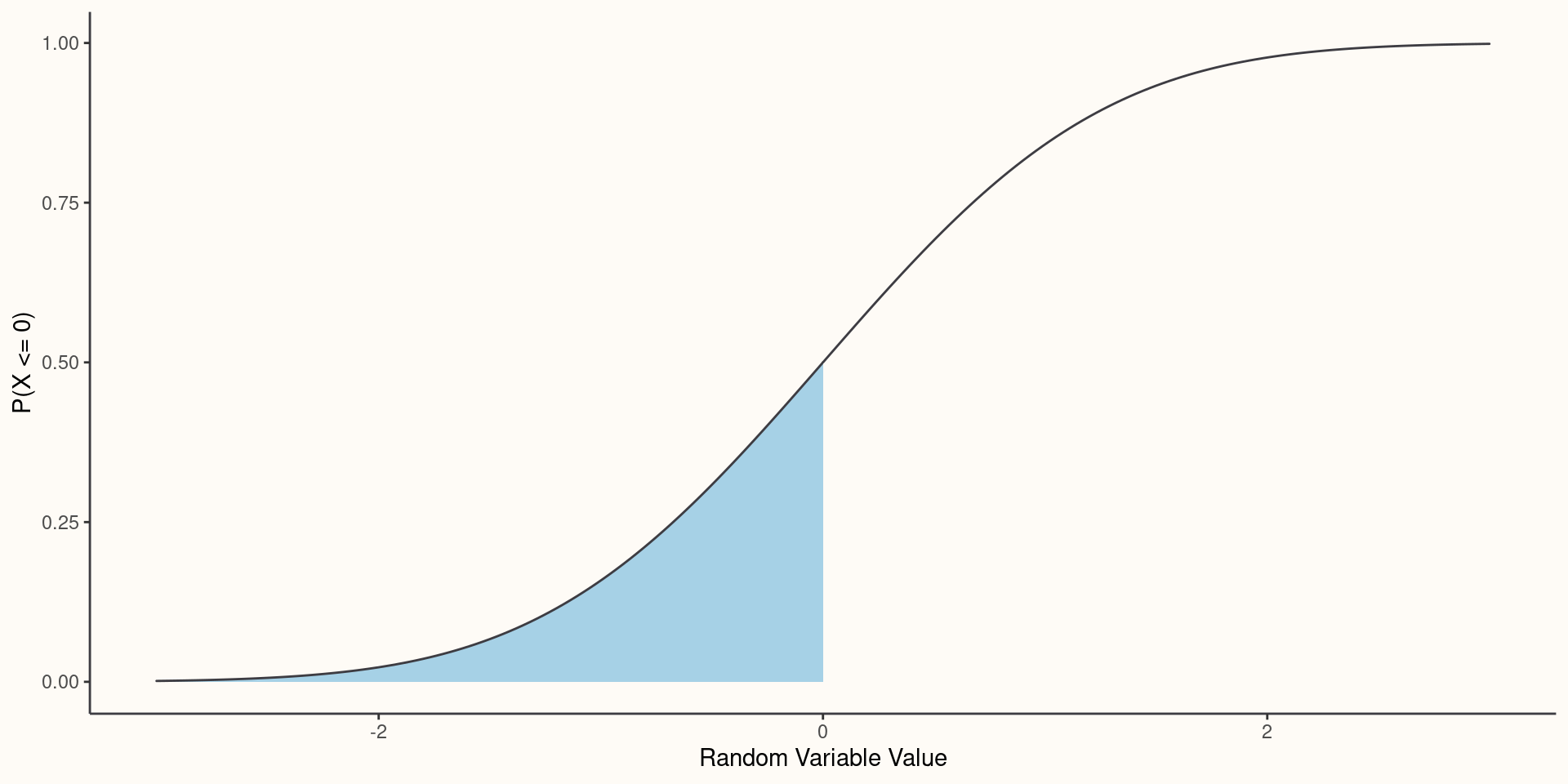
Normal PDF

Normal CDF

Bivariate Relationships

• We can use PMFs / PDFs and CDFs to describe the probabilistic relationship between two random variables:
  • Joint PMF: \(f(x, y)=P(X = x, Y = y)\)
  • Joint CDF: \(F(x,y) = P(X \leq x, Y \leq y)\)
  • Marginal PMF: \(f_{Y}=P(Y = y) = \sum_{x}f(x,y)\)
  • Conditional PMF: \(f_{Y|X}(y|x)=\frac{P(Y = y, X = x)}{P(X = x)}=\frac{f(x,y)}{f_{x}(x)}\)

Summarizing Distributions

• We often need to summarize the information contained in marginal and joint distributions. We can do this using several different summary measures:

  • Expectation Operator, \(E[X]\), provides us with information about the center of the distribution.
  • Variance, \(E[(X-E[X])^{2}]\), provides us with information about the shape of the distribution.
  • Covariance, \(E[(X - E[X])(Y - E[Y])]\), provides us with information about how X and Y move together.
  • Conditional Expectation, \(E[Y|X]\), provides us with information about \(E[Y]\) given X occurred.

Expectation Operator

• The expectation, \(E\), of a random variable is the value we would get if we took the mean over an infinite number of realizations of a random variable (if we conducted the same experiment an infinite number of times).

• The expectation operator is a function that takes a random variable as an input and outputs a real number, the expected value of random number: \(E[X]=\sum_{x}xf_{x}(x)\).

• Some useful properties:

  • \(E[c]=c\) if \(c\) is a constant
  • \(E[aX]=aE[X]\) if \(a\) is a constant
  • \(E[aX + c]=aE[X] + c\)—Linearity of Expectations

Variance & Standard Deviation

• The variance, \(\sigma^{2}\), of a random variable tells us about the spread of its distribution. The larger the variance the more unpredictable the random variable.

• The standard deviation, \(\sigma\), is the square root of the variance. It gives us the same information as the variance, but the standard deviation can be interpreted using the scaling of the random variable.

• Some useful properties:

  • \(V[X]=E[X^{2}] - E[X]^{2}\)—an easier formula to compute the variance
  • \(V[c] = 0\) if c is a constant
  • \(V[X + c]= V[X]\) if c is a constant
  • \(V[aX]=a^{2}V[X]\) if a is a constant
  • \(V[X + Y]=V[X]+V[Y]+2Cov[X, Y]\)—variance of a sum score (this will come in handy when we talk about reliability)

Covariance & Correlation

• The positive covariance between two variables, X and Y, tells us if large values of X tend to occur with large values of Y (and small with small).

• The negative covariance tells us if large values of X tend to occur with small values of Y and if small values of X tend to occur with large values of Y.

• The correlation is just the standardized version of covariance: \(\frac{Cov[X, Y]}{\sigma_{x}\sigma_{y}}\)

• Some useful properties:

  • \(Cov[X, Y]=E[X, Y] - E[X]E[Y]\)—easier to compute
  • \(Cov[X, c]=0\) if c is a constant
  • \(Cov[X, Y] = Cov[Y, X]\)—covariance is symmetrical
  • \(Cov[X, X]=V[X]\)—the covariance of a variable with itself is its variance
  • \(Cov[aX + b, cY + d] = acCov[X, Y]\) if a, b, c, and d are constants

Conditional Expectation

• The conditional expectation of a random variable, \(E[Y|X=x]\), tells us the expected variable of one random variable given the value of another random variable.

• Conditional expectations allow us to describe how the expected variable of one variable changes once we condition on the observed value of another random variable. This is exactly what linear regression does!

• Some useful properties:

  • \(E[h(x,y)|X=x]=\sum_{y}h(x,y)f_{Y|X}(y|x)\)—Conditional expectation of a function
  • \(E[g(X)Y|X=x]=g(x)E[Y|X=x]\)—Functions of X, \(g(X)\), are treated as constants
  • \(E[g(X)Y+h(X)|X=x]=g(x)E[Y|X=x]+h(x)\)—Linearity of Conditional Expectations

Samples Instead of Populations

• Every statistical model we will use assumes that our sample data are independently and identically distributed—the iid assumption.

• The iid assumption is basically a simplifying assumption that assumes two things:

  • One observation of a random variable cannot give us any information about another observation of that same random variable (e.g. knowing my score on the selection assessment tells us nothing about Ben’s score).
  • Our data all came from the same joint (marginal) probability distribution.

Sample Statistics

• The goal of statistical inference is to estimate population parameters (like the mean and variance) of a population distribution from a sample. Sample statistics allow us to accomplish this goal.

• Sample statistics are functions of our sample data that estimate some feature of a random variable’s population distribution:

  • Sample Mean, \(\bar{X}=\frac{\sum{X}}{n}\), estimates the population mean, \(\mu=E[X]\)
  • Sample Variance, \(\hat{\sigma}=\frac{\sum{(X - \bar{X})^2}}{n-1}\), estimates the population variance, \(\sigma^2\)
  • Estimated Regression Coefficient, \(\hat{\beta}\), estimates the population regression coefficient, \(\beta\)

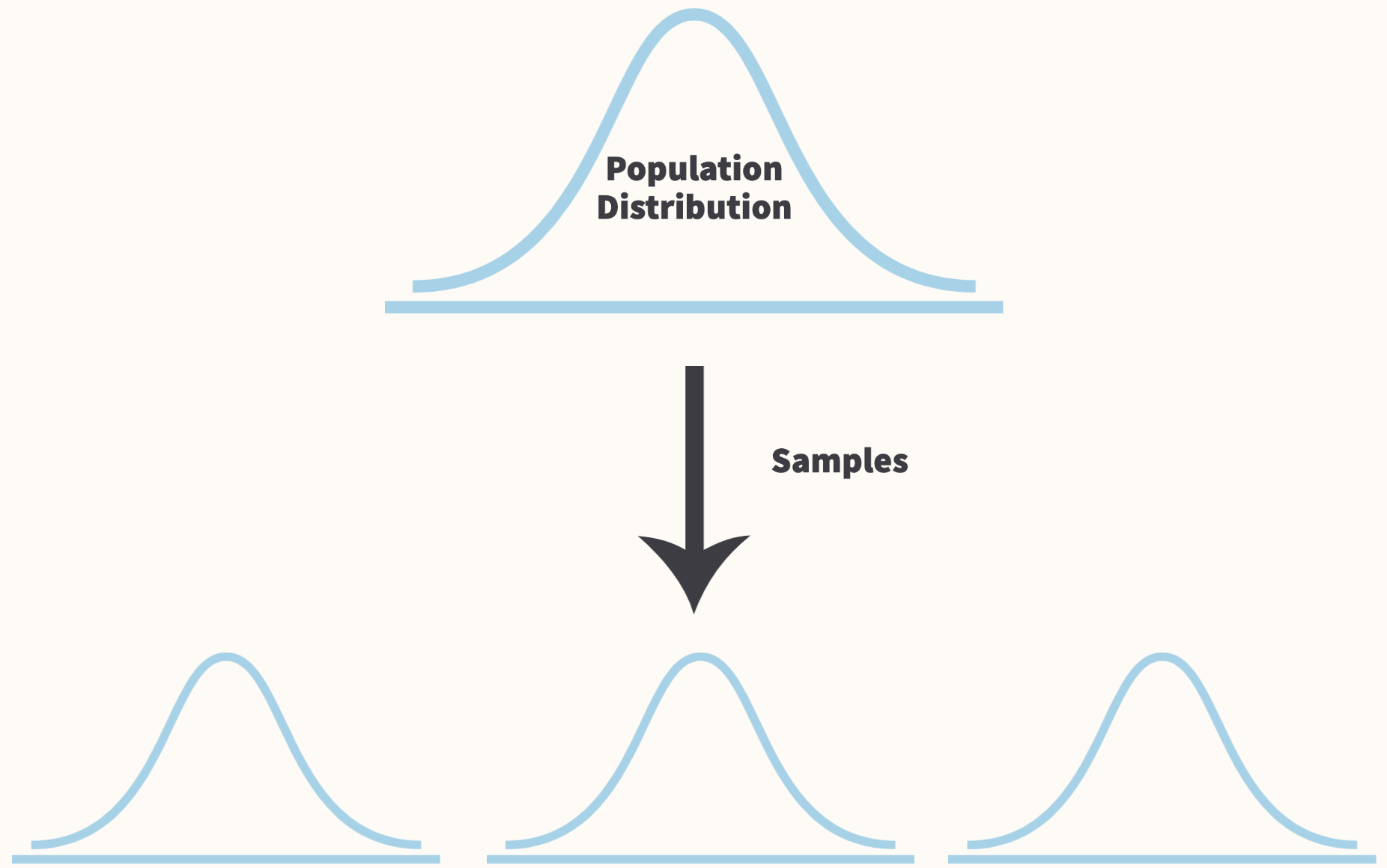
Sampling Distributions

• Because a sample statistics is a function of a random variable, it is therefore also a random variable with its own distribution: Sampling Distribution.

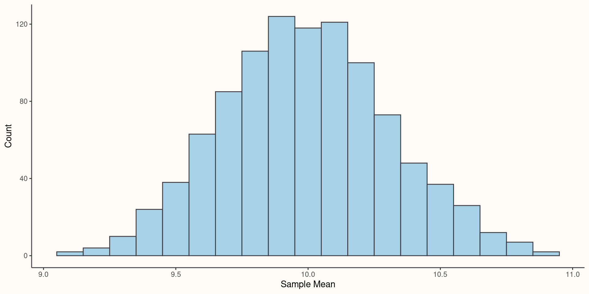
• Imagine drawing 1,000 iid samples of applicant scores on a selection assessment. For each sample you compute the sample mean. You could approximate the sampling distribution of the mean by making a histogram using the 1,000 sample means you computed.

  • The mean of those 1,000 means would be equal (or close to) the population mean of the selection assessment scores.
    
  • The standard deviation of those 1,000 means would equal something called the standard error of the estimate (the standard error of the mean), which tells us how much uncertainty is in our estimate.

Sampling Distribution Simulation

set.seed(42)
population_mean <- 10
population_variance <- 5
number_samples <- 1000
sample_size <- 50
sample_mean <- numeric()

for(i in 1:number_samples) {
  x <- rnorm(
    n = sample_size, 
    mean = population_mean,
    sd = sqrt(population_variance)
  )
  
  sample_mean_1 <- mean(x)
  sample_mean <- 
    c(sample_mean, 
      sample_mean_1)
}

mean(sample_mean) # Should be close to the population mean

[1] 9.993821

sd(sample_mean) # Standard Error of the Mean

[1] 0.3151269

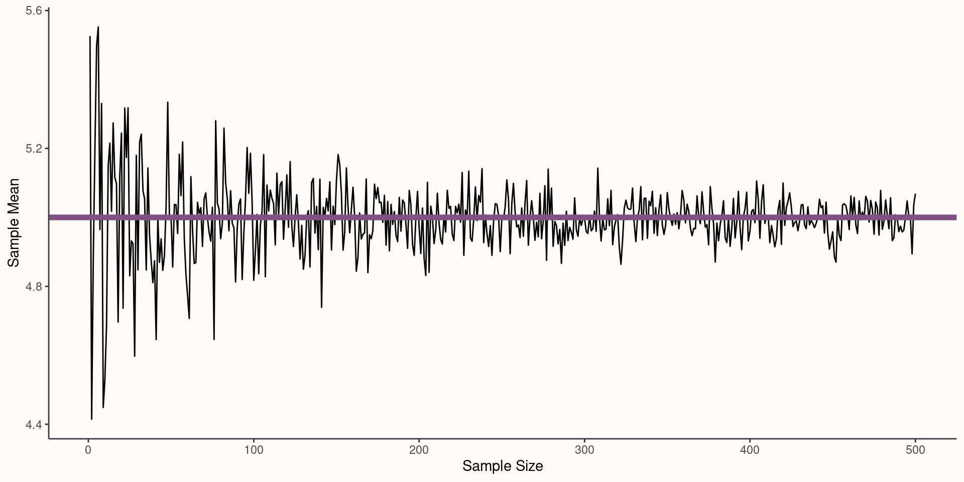
Weak Law of Large Numbers

mean_plot_data <- 
  data.frame(
    N = 1:500,
    SAMPLE_MEAN = NA
  )

for(n in 1:500) {
  
  sample_mean <- 
    rnorm(n = n, mean = 5, sd = 1) |>
    mean()
  
  mean_plot_data[n, 2] <- sample_mean
  
  
}

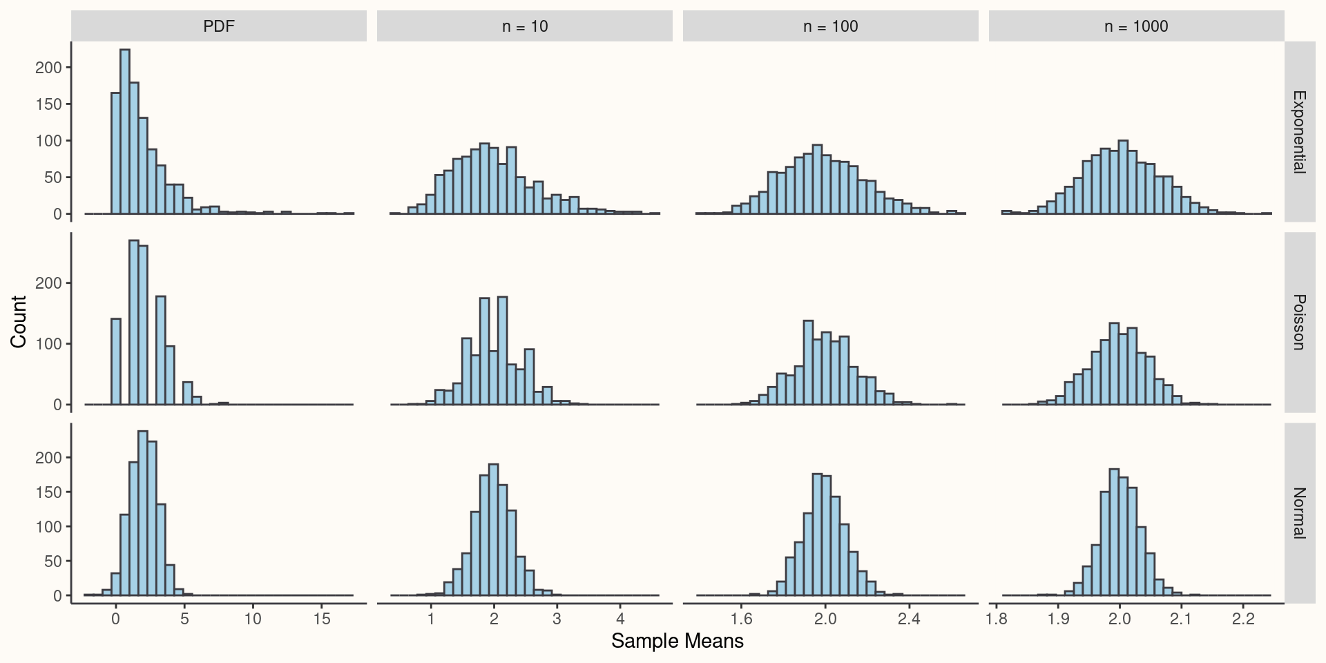
Central Limit Theorem

• The Central Limit Theorem proves that the sampling distribution of an estimate created by averaging many (\(n \approx 30\)) iid random variables will tend to be approximately normal as \(n\) increases even if the underlying distribution of the iid variables is not normal.

\[Z = \frac{\bar{X}-E[X]}{SE_{\bar{X}}}=\frac{\sqrt{n}(\bar{X}-\mu)}{\sigma}\]

\[Z \xrightarrow{d} N(0, 1)\]

Central Limit Theorem Visualized

Statistical Inference: Two Questions

• Statistical inference asks two broad questions:
  • What is the value of an unknown parameter and how do we quantify uncertainty about the estimate?
  • How consistent are the data with a stated claim or hypothesis about the value of a parameter?

Population Example

• We have all the tools we need to start making inferences from the data to the population!

• Example: Here is the population model we will be making inferences about:

\[Y = \beta_{0}+\beta_{1}X_{1}+\beta_{2}X_{2}+\epsilon\]

\[\epsilon \sim N(0, \sigma^{2})\]

• \(Y =\) Job Performance, \(X_{1} =\) Structured Interview, and \(X_{2} =\) Graphology

Drawing Inferences from our Data

# Set the parameters 
set.seed(32) # Seed for reproducibility
n <- 500 # Sample size
b0 <- 2 # Population Regression Intercept
b1 <- 1 # Population Regression Slope
sigma <- 4 # Population variance

x1 <- sample(
  1:5, 
  size = n, 
  replace = TRUE, 
  prob = c(.10, .15, .15, .30, .30)
)

x2 <- sample(
  1:5,
  size = n,
  replace = TRUE
)

# Generate dependent var.
y <- rnorm(
  n = n, 
  mean = b0 + b1*x1 + 0*x2, 
  sd = sqrt(sigma)
) 

mod <- lm(y ~ x1 + x2) # Estimate model 

Call:
lm(formula = y ~ x1 + x2)

Residuals:
    Min      1Q  Median      3Q     Max 
-5.9736 -1.3566 -0.0707  1.3735  7.1174 

Coefficients:
            Estimate Std. Error t value Pr(>|t|)    
(Intercept)  1.68456    0.32556   5.174 3.32e-07 ***
x1           0.95949    0.06873  13.960  < 2e-16 ***
x2           0.11486    0.06581   1.745   0.0815 .  
---
Signif. codes:  0 '***' 0.001 '**' 0.01 '*' 0.05 '.' 0.1 ' ' 1

Residual standard error: 2.034 on 497 degrees of freedom
Multiple R-squared:  0.2859,    Adjusted R-squared:  0.283 
F-statistic: 99.48 on 2 and 497 DF,  p-value: < 2.2e-16

Conducting Statistical Inference

• How would you use the model output?

Call:
lm(formula = y ~ x1 + x2)

Residuals:
    Min      1Q  Median      3Q     Max 
-5.9736 -1.3566 -0.0707  1.3735  7.1174 

Coefficients:
            Estimate Std. Error t value Pr(>|t|)    
(Intercept)  1.68456    0.32556   5.174 3.32e-07 ***
x1           0.95949    0.06873  13.960  < 2e-16 ***
x2           0.11486    0.06581   1.745   0.0815 .  
---
Signif. codes:  0 '***' 0.001 '**' 0.01 '*' 0.05 '.' 0.1 ' ' 1

Residual standard error: 2.034 on 497 degrees of freedom
Multiple R-squared:  0.2859,    Adjusted R-squared:  0.283 
F-statistic: 99.48 on 2 and 497 DF,  p-value: < 2.2e-16

What are P Values?

• The P value is a statistical summary of the compatibility between the observed data and what we would predict or expect to see if we knew the entire statistical model were correct.

\[\text{P value} = P(Data|Model)\]

• Most statistical programming languages report a P value based on the assumption that the effect under investigation is equal to 0.

• The P value of 0.082 for \(X_{2}\) can be interpreted as: “Assuming all of our model assumptions are true including no effect of \(X_{2}\), the probability of seeing a value as or more extreme than 0.115 is 0.082.

Computing P Values

• We can compute a P value for any null hypothesis not just a null hypothesis of 0 effect. We just need four things:
  • Estimated effect
  • Estimated standard error for the effect
  • Value of the null hypothesis
  • Model degrees of freedom
• Using these four pieces of information, we can construct our test statistic and P value:

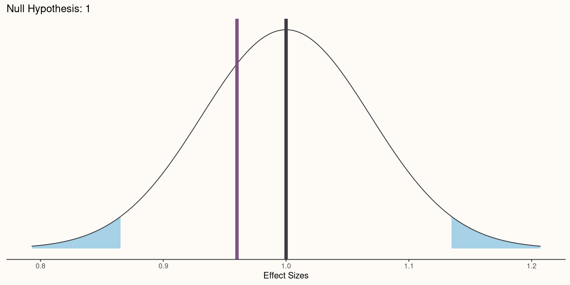
\[T = \frac{Est. - H_{0}}{SE_{est.}}\]

\[\text{P Value}=2\times P(|T| \geq|t| \mid H_{0}=True, Model = True) \]

Visualizing P Values

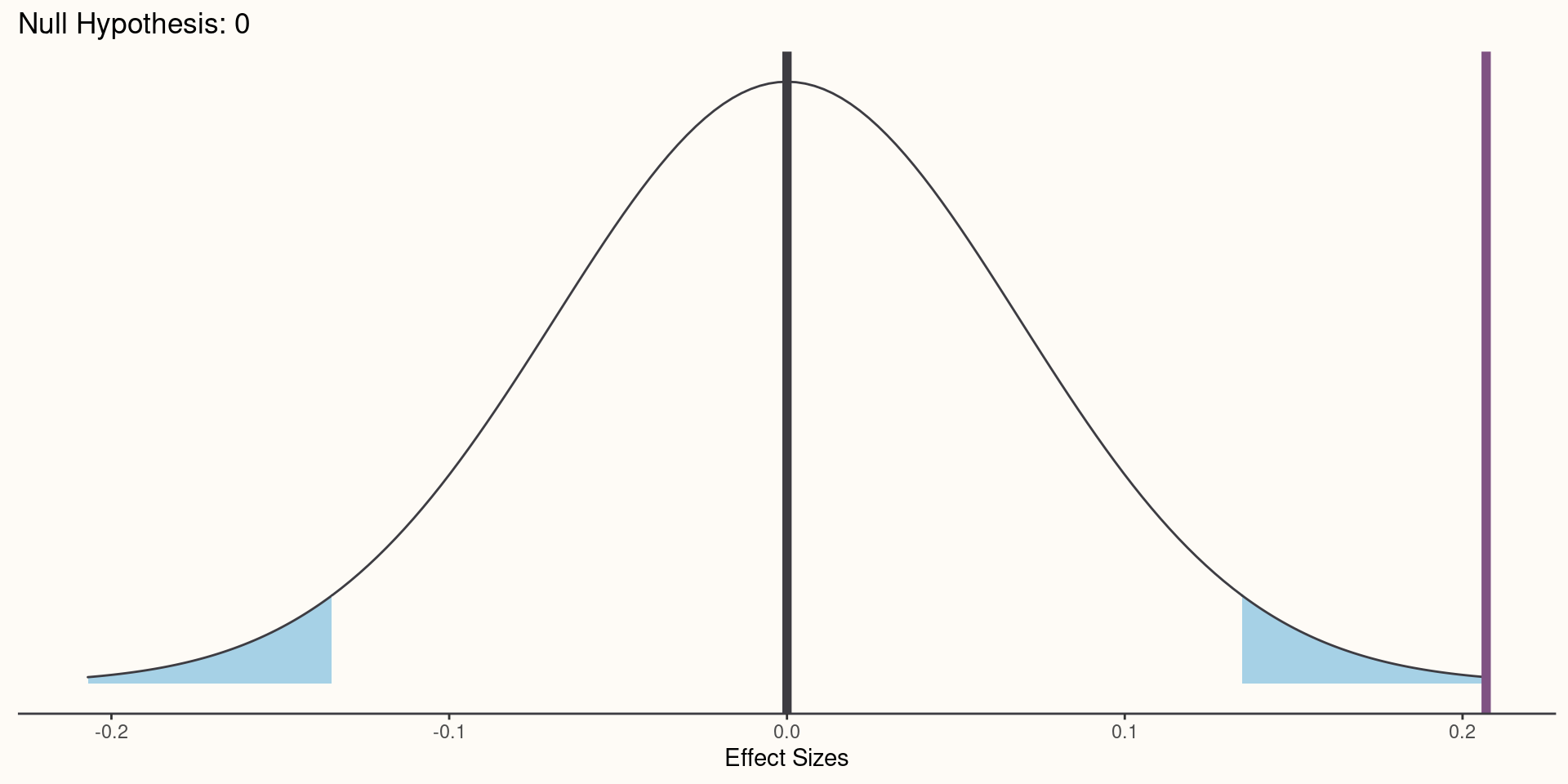
Visualizing P Values

Coding P Values

# X2 coefficient and SE
x2_beta <- summary(mod)$coef[3, 1]
x2_se <- summary(mod)$coef[3, 2]

# Test statistics
test_stat_0 <- (x2_beta - 0) / x2_se # Null = 0
test_stat_25 <- (x2_beta - .25) / x2_se # Null = .25

# P-value for x2 when null hypothesis = 0 (using a central T distribution)
pnorm(abs(test_stat_0), mean = 0, sd = 1, lower.tail = FALSE) * 2 |>
  round(3)

[1] 0.08092986

# P-value for x2 when null hypothesis = .25
pnorm(abs(test_stat_25), mean = 0, sd = 1, lower.tail = FALSE) * 2 |>
  round(3)

[1] 0.04001684

Confidence Intervals: Two Interpretations

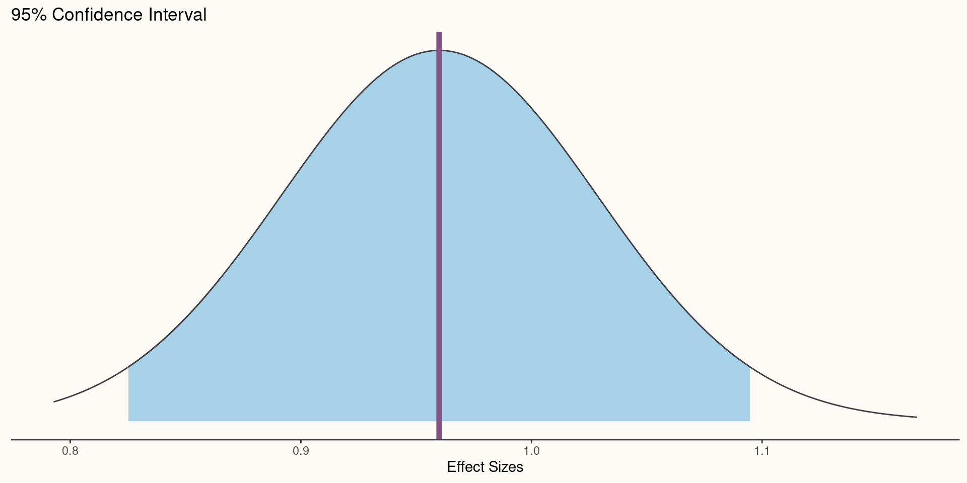
• Confidence interval: A range of effect sizes whose tests produced \(\text{P Value}\gt .05\) and thus are considered to be more compatible with the data compared to effect sizes outside of the interval GIVEN that the model and its assumptions are all correct.

• Confidence Interval: A range of values that contain the population value, estimated by a sample statistic (e.g. regression coefficient), with a given probability—usually 95%.

\[P(\hat{\beta}-SE_{\hat{\beta}}\times C\leq\beta\leq\hat{\beta}+SE_{\hat{\beta}}\times C)=.95\]

• \(C\) is usually set equal to 1.96 to create a normal distribution approximation.

Visualizing a Confidence Interval

Confidence Interval: Interpretation 1

confint_mod <- confint(mod) # Creates 95% confidence intervals
x1_coef <- summary(mod)$coef[2, 1]
x1_se <- summary(mod)$coef[2, 2]
x1_lower <- confint_mod[2, 1]
x1_upper <- confint_mod[2, 2]
x1_lower_pvalue <- pnorm(x1_coef, mean = x1_lower, sd = x1_se, lower.tail = F)*2
x1_upper_pvalue <- pnorm(x1_coef, mean = x1_upper, sd = x1_se, lower.tail = T)*2

# A tibble: 1 × 6
  X1_COEF X1_STD_ERROR X1_LOWER_CI X1_UPPER_CI X1_LOWER_P X1_UPPER_P
    <dbl>        <dbl>       <dbl>       <dbl>      <dbl>      <dbl>
1   0.959        0.069       0.824        1.10      0.049      0.049

Confidence Interval: Interpretation 2

# Set the parameters 
set.seed(3342) # Seed for reproducibility
n <- 500 # Sample size
b0 <- 2 # Population Regression Intercept
b1 <- 1 # Population Regression Slope
sigma <- 4 # Population variance

x1 <- sample(
  1:5, 
  size = n, 
  replace = TRUE, 
  prob = c(.10, .15, .15, .30, .30)
)

x2 <- sample(
  1:5,
  size = n,
  replace = TRUE
)

ci_vec <- numeric() # Create CI vector
for(i in 1:500) {
  
  # Generate dependent var.
  y <- rnorm(
  n = n, 
  mean = b0 + b1*x1 + 0*x2, 
  sd = sqrt(sigma)
) 
  
  mod <- lm(y ~ x1 + x2) # Estimate model 
  
  # Get CI
  ci_mod <- confint(mod)
  ci_lower <- ci_mod[2, 1]
  ci_upper <- ci_mod[2, 2]
  
  # Does CI contain pop. par -- Yes or No
  coverage <- ci_lower <= b1 & b1 <= ci_upper
  ci_vec <- c(ci_vec, coverage)
  
}

# What proportion of CIs contained pop. par.?
mean(ci_vec)

[1] 0.946