Item Response Theory

Overview

Comparison of IRT to CTT and factor analysis
Overview of dichotomous IRT models
Overview of IRT model testing

What is IRT?

IRT is a measurement theory that uses generalized linear latent variable models to model the response to a binary item.
Unlike CTT or GT, which model aggregated (sum score and mean score, respectively) item scores, IRT is focused on the individual items that make up a test.

How does IRT differ from CTT?

In IRT:
- Item parameters such as item difficulty and item discrimination are invariant to the respondent population.
- The standard error of measurement (and reliability) is conditional on the ability of a respondent.
- Estimates of an individuals theta (ability / latent variable) are not confounded with item parameter estimates.
Cost of IRT:
- Stronger modeling assumptions.

How do IRT Models differ from Factor Analysis Models?

Think of factor analysis as analogous to linear regression with a latent (unobserved) predictor and IRT as analogous to logistic regression with a latent predictor.
Use IRT models to model responses to binary items.

Applications of IRT

Educational measurement
- Cognitive tests: GRE & SAT (right / wrong responses)
Attitude measurement
- Likert scales with less than 5 responses
- Binary agreement scales
- Ideal point models
Personality measurement
- Binary agreement scales

Item Response Function

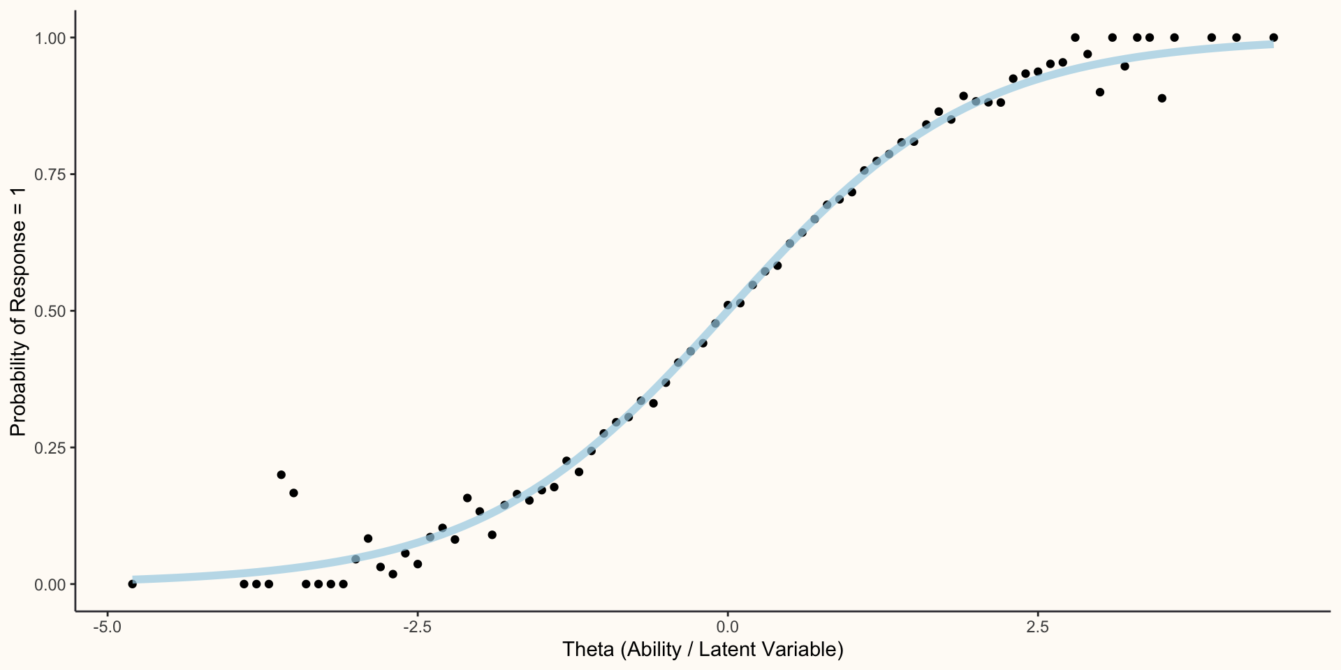
The item response function is any function that describes the probability of correctly responding to an item as a monotonically increasing function of theta (someone’s ability).

IRT Models

When analyzing binary data, IRT has typically relied on a class of item response functions called the logistic functions:

\[P(X = 1)=\frac{e^{f(\Theta_{i})}}{1 + e^{f(\Theta_{i})}}=\frac{1}{1 + e^{-f(\Theta_{i})}}\]

The logistic functions have been further classified based on the number of parameters they use to model the item response: 1PL, 2PL, 3PL, and 4PL

One Parameter Logistic Model

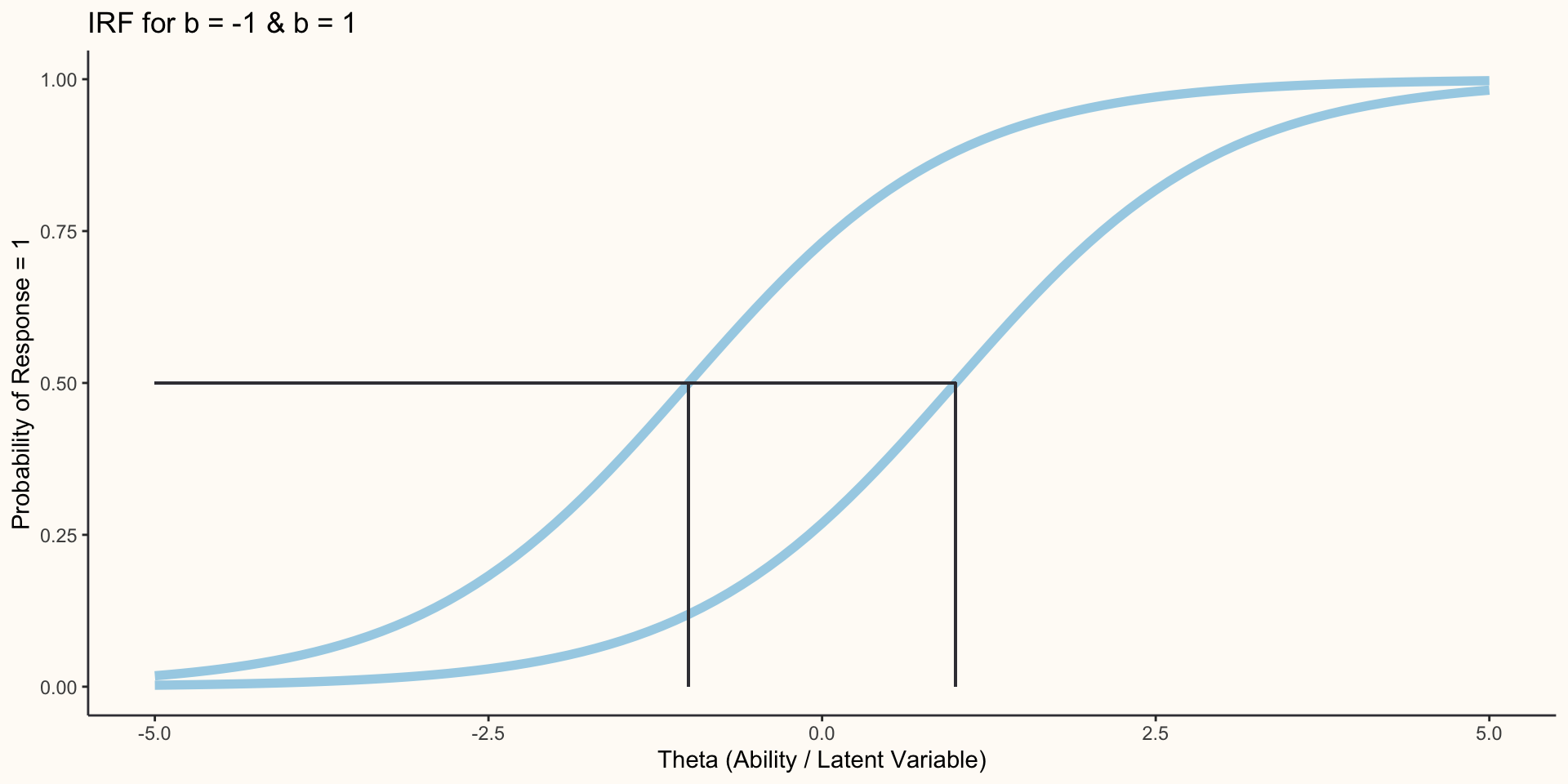
The one parameter logistic (1PL) model describes an individual’s item response using only a single parameter: b. The discrimination parameter, a, is a constrained parameter.
b is the difficulty parameter, it tells us how difficult the item is (for cognitive tests) or what level of theta is needed (attitude measurements) for an individual to respond 1 to the item:

\[P(X = 1)=\frac{1}{1 + e^{-a(\Theta_{i}-b_{j})}}\]

1PL Iten Response Function

Rasch Models: A Quick Aside

Rasch Models = 1PL Model with a (discrimination parameter set equal to 1 for all items).
Although Rasch models can be equivalent to the 1PL model, Rasch models are less of a theory of measurement and more of an ideology of measurement.
IRT (Logistic models) tries to build models that best describe the item responses (descriptive model of item response), whereas Rasch models try to build items that fit the Rasch model (normative model of item response).

Two Parameter Logistic Model

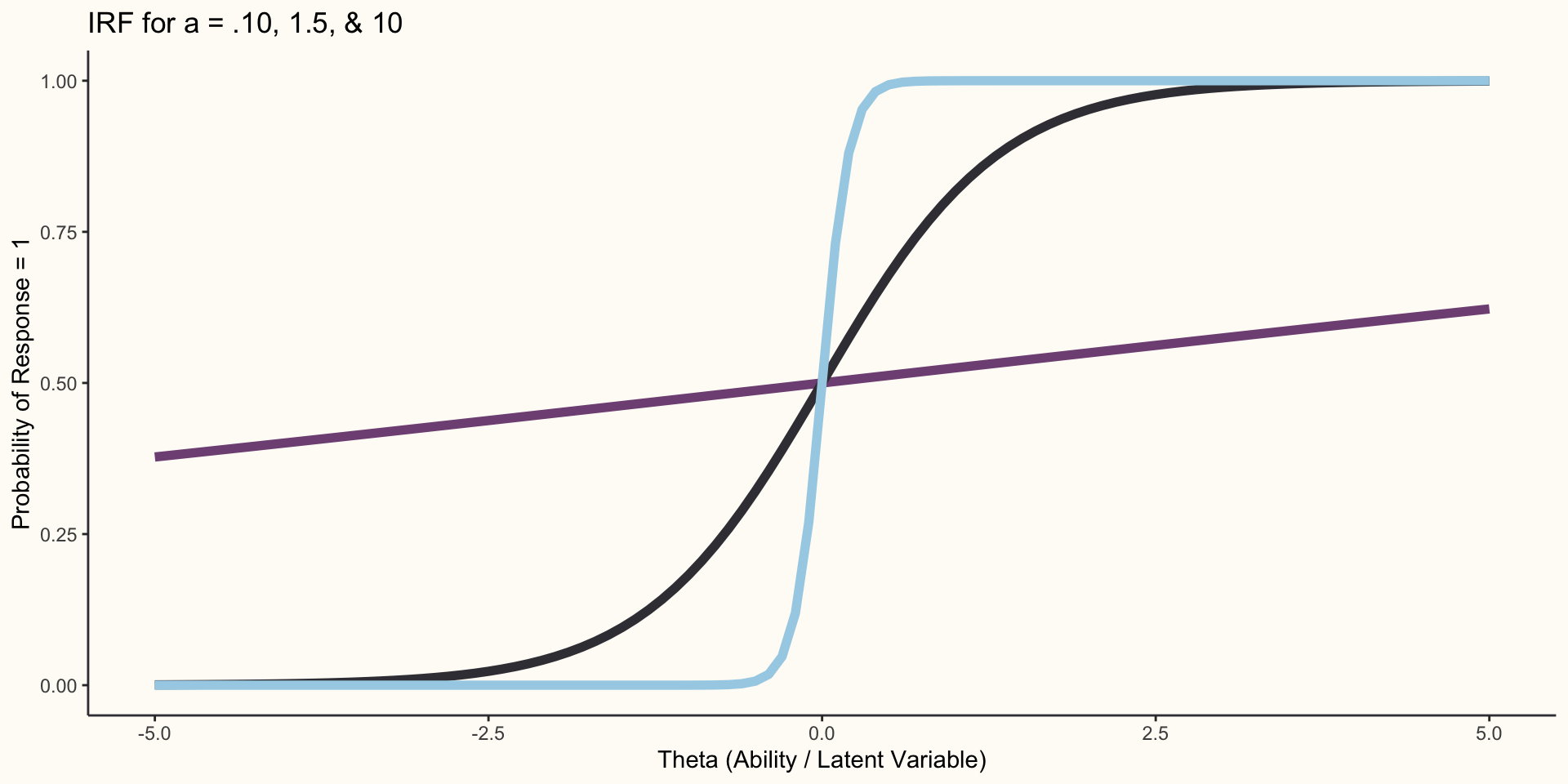
The 2PL is equivalent to the 1PL except now the discrimination parameter, a, is freely estimated for each item:

\[P(X = 1)=\frac{1}{1 + e^{-a_{j}(\Theta_{i}-b_{j})}}\]

The discrimination parameter tells us how well a given item can differentiate among respondents with differing levels of theta.

2PL Item Response Function

Three Parameter Logistic Model

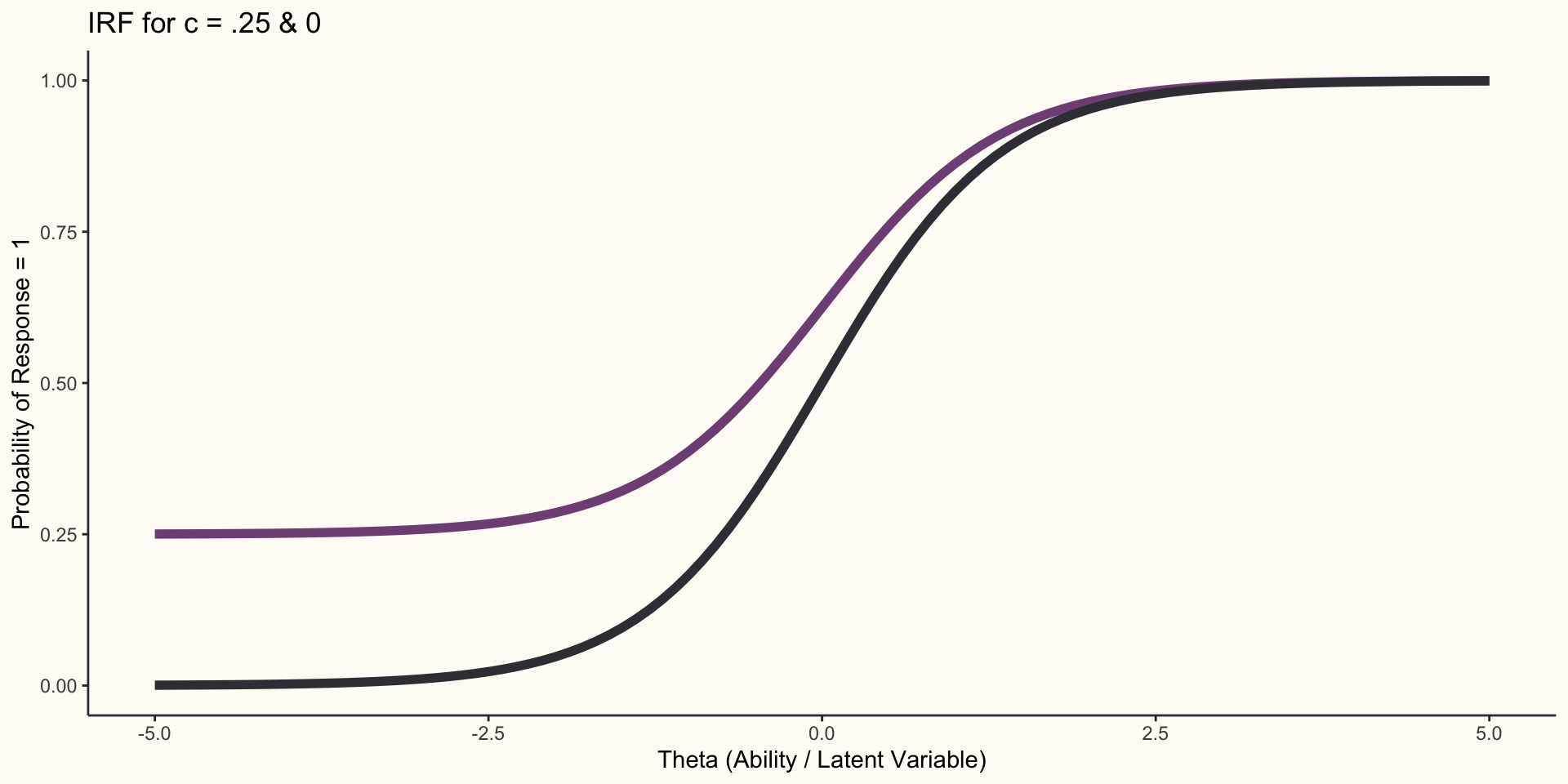
The 3PL is equivalent to the 2PL model with an additional parameter added, c, the guessing parameter, which had previously been constrained to 0:

\[P(X = 1)=c_{j} + (1 - c_{j})\frac{1}{1 + e^{-a_{j}(\Theta_{i}-b_{j})}}\]

The guessing parameter, c, changes the lower asymptote of the IRF from 0 to c.

3PL Item Response Function

Four Parameter Logistic Model

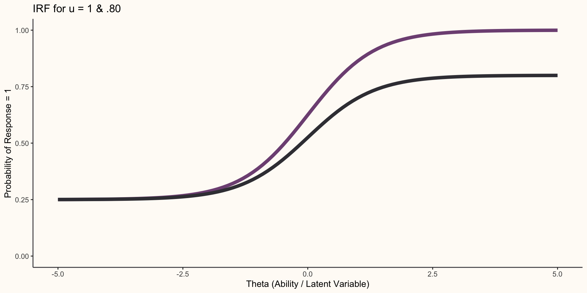
The 4PL is equivalent to the 3PL model with an additional parameter added, u, the upper limit, which had previously been constrained to 1:

\[P(X = 1)=c_{j} + (u_{j} - c_{j})\frac{1}{1 + e^{-a_{j}(\Theta_{i}-b_{j})}}\]

The upper limit parameter, u, changes the upper asymptote of the IRF from 1 to u.

4PL Item Response Function

Estimating IRT Logistic Parameter Models with R

There are two main R packages for estimating IRT logistic models:
- ltm
- mirt

A Glimpse of Our Data

# A tibble: 6 × 15
  ITEM_1 ITEM_2 ITEM_3 ITEM_4 ITEM_5 ITEM_6 ITEM_7 ITEM_8 ITEM_9 ITEM_10 ITEM_11
   <int>  <int>  <int>  <int>  <int>  <int>  <int>  <int>  <int>   <int>   <int>
1      0      1      1      0      0      0      0      1      0       0       0
2      0      0      1      1      0      0      0      0      0       1       0
3      1      1      1      1      0      0      1      0      0       0       0
4      0      1      1      1      1      0      0      1      1       0       0
5      0      1      1      1      0      1      1      1      1       1       1
6      1      0      1      1      0      0      0      1      1       0       0
# … with 4 more variables: ITEM_12 <int>, ITEM_13 <int>, ITEM_14 <int>,
#   ITEM_15 <int>

Estimating the 2PL Model with `mirt`

twopl_mod <- "F = ITEM_1-ITEM_15"

twopl_fit <- mirt(data = twopl_df, model = twopl_mod,
                  itemtype = "2PL", SE = TRUE, verbose = FALSE)

twopl_params <- coef(twopl_fit, IRTpars = TRUE, simplify = TRUE)

Examining Item Parameters

$items
            a      b g u
ITEM_1  0.991  1.164 0 1
ITEM_2  0.814  0.552 0 1
ITEM_3  1.506  0.022 0 1
ITEM_4  1.232 -1.354 0 1
ITEM_5  0.710  0.972 0 1
ITEM_6  1.077  0.446 0 1
ITEM_7  1.561  0.588 0 1
ITEM_8  0.814  0.293 0 1
ITEM_9  1.895 -0.024 0 1
ITEM_10 1.067  1.336 0 1
ITEM_11 0.750  0.705 0 1
ITEM_12 0.893  0.076 0 1
ITEM_13 1.161  0.484 0 1
ITEM_14 1.526 -1.319 0 1
ITEM_15 1.102  0.536 0 1

$means
F 
0 

$cov
  F
F 1

Benefits of IRT

Item Parameter Invariance
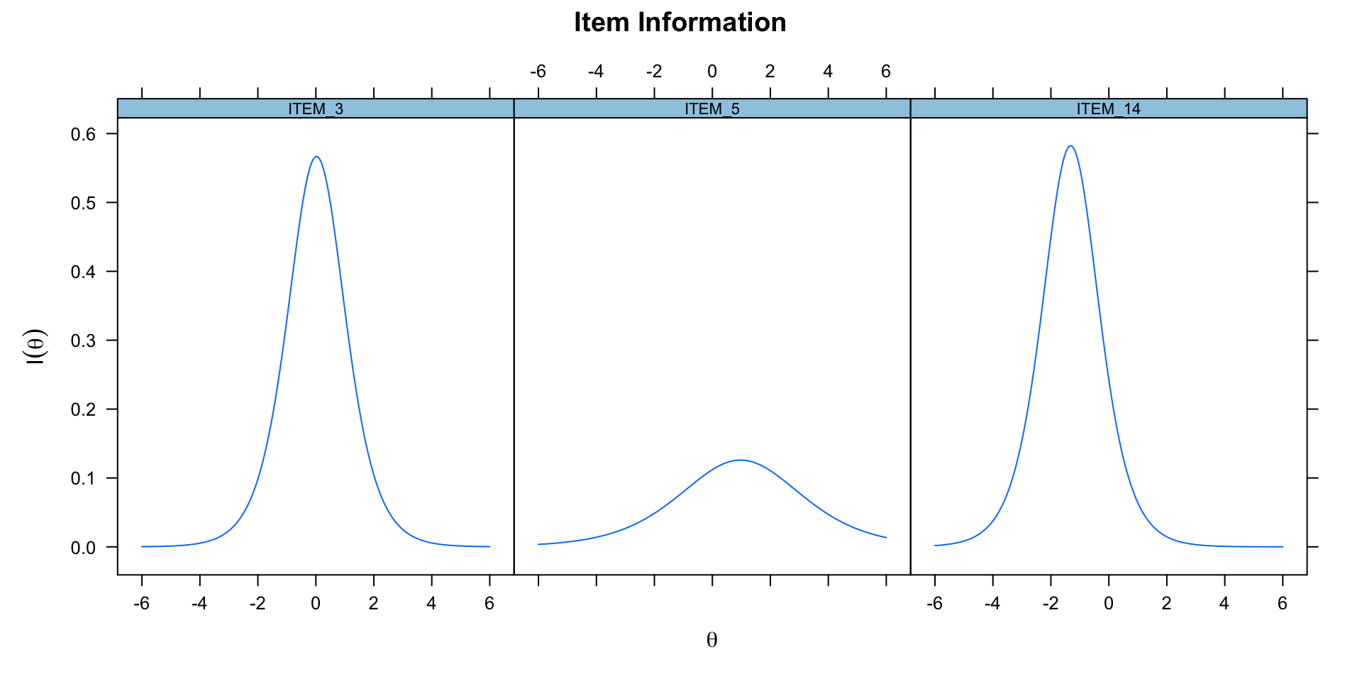
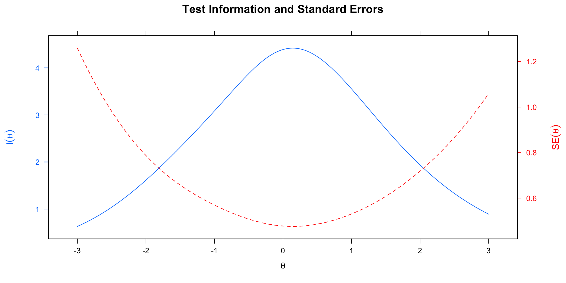
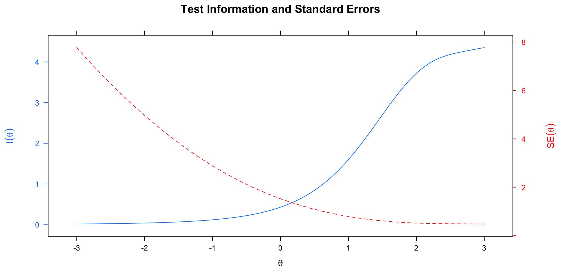
Conditional Standard Errors of Measurement (Item information)
- Our items (and tests) can be better at measuring different levels of theta

Item Information

plot(twopl_fit, type = "infotrace", which.items = c(3, 5, 14))

Test Information

Test Information At High Levels of Theta

IRT Assumptions

(Unidimensional) IRT makes the following three assumptions:
- Unidimensionality
- Local Independence
- Correct Functional Form

Unidimensionality

Unidimensional IRT requires that each item measure one and only one dimension. There is a multidimensional extension of IRT, but we will not cover that here.
You can test unidimensionality using several different methods:
- Scree plot
- Horns Parallel Analysis
- Model testing using mirt

Horns Parallel Analysis

# Calculate tetrachoric correlation matrix
twopl_cor <- psych::tetrachoric(twopl_df)

# Horns Parallel Analysis
psych::fa.parallel(
  x = twopl_cor$rho,
  cor = "tet",
  n.obs = 2000, 
  fa = "pc",
  fm = "ml"
)

Parallel Analysis Results

Parallel analysis suggests that the number of factors =  NA  and the number of components =  1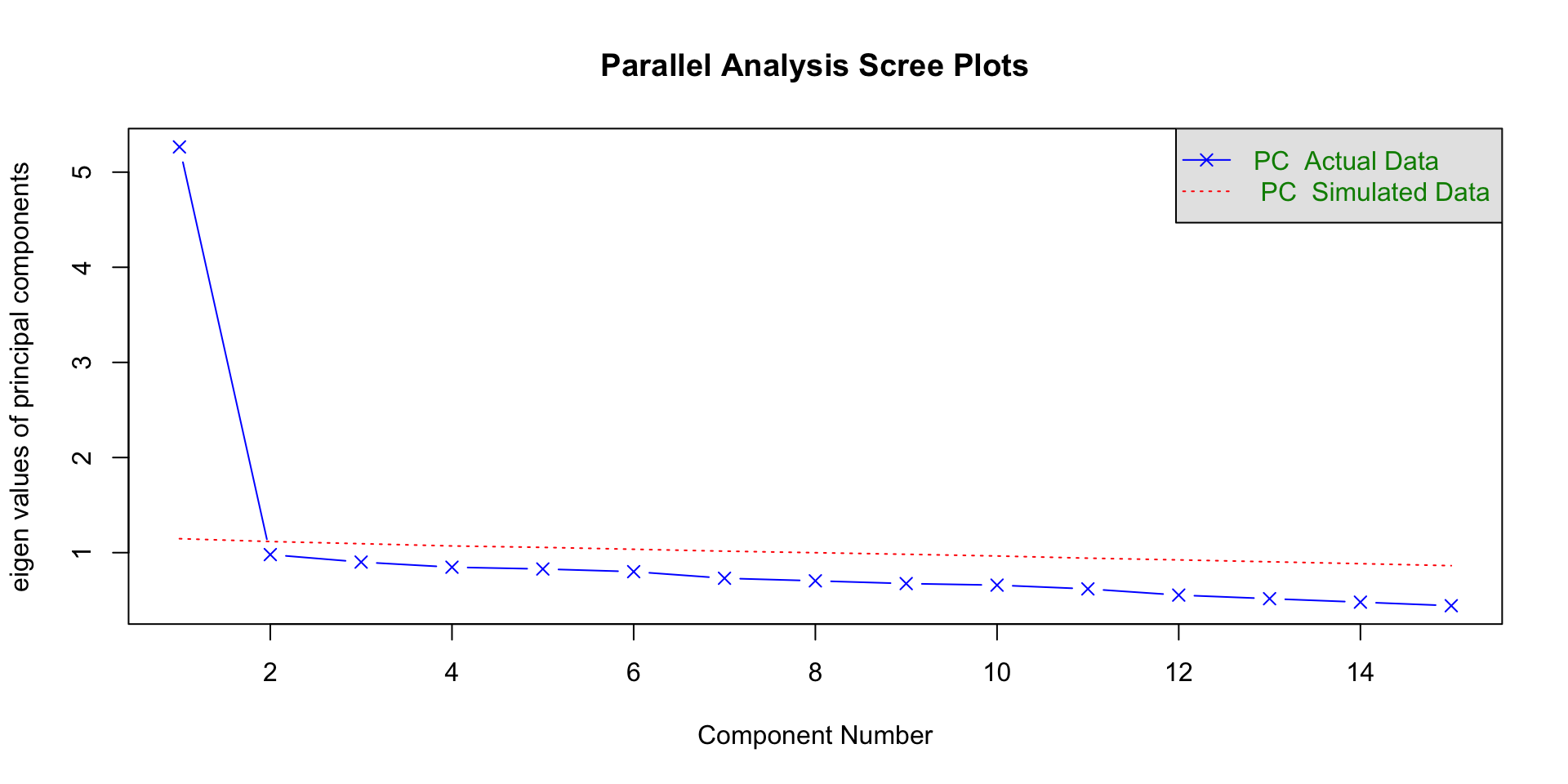

Local Independence

Local independence is the assumption that once you control for theta, there should be no remaining correlation among the items. That is, if we look at a group of individuals with very high levels of theta, the item responses should not correlate.
Local independence & Unidimensionality are very similar assumptions–if unidimensionality holds, then local independence should hold as well.
Yen’s Q3 Statistic estimates the correlations among the item residuals

Testing Local Independence

mirt::residuals(twopl_fit, type = "Q3")

Q3 summary statistics:
   Min. 1st Qu.  Median    Mean 3rd Qu.    Max. 
 -0.162  -0.076  -0.055  -0.056  -0.028   0.009 

        ITEM_1 ITEM_2 ITEM_3 ITEM_4 ITEM_5 ITEM_6 ITEM_7 ITEM_8 ITEM_9 ITEM_10
ITEM_1   1.000 -0.053 -0.083 -0.027 -0.006 -0.017 -0.131  0.004 -0.059  -0.080
ITEM_2  -0.053  1.000 -0.074 -0.061 -0.065 -0.025 -0.040 -0.012 -0.069  -0.005
ITEM_3  -0.083 -0.074  1.000 -0.044 -0.033 -0.063 -0.111 -0.048 -0.137  -0.088
ITEM_4  -0.027 -0.061 -0.044  1.000 -0.028 -0.085 -0.042 -0.062 -0.068  -0.029
ITEM_5  -0.006 -0.065 -0.033 -0.028  1.000 -0.019 -0.072 -0.042 -0.079  -0.028
ITEM_6  -0.017 -0.025 -0.063 -0.085 -0.019  1.000 -0.082 -0.051 -0.102  -0.048
ITEM_7  -0.131 -0.040 -0.111 -0.042 -0.072 -0.082  1.000 -0.065 -0.162  -0.055
ITEM_8   0.004 -0.012 -0.048 -0.062 -0.042 -0.051 -0.065  1.000 -0.085  -0.072
ITEM_9  -0.059 -0.069 -0.137 -0.068 -0.079 -0.102 -0.162 -0.085  1.000  -0.078
ITEM_10 -0.080 -0.005 -0.088 -0.029 -0.028 -0.048 -0.055 -0.072 -0.078   1.000
ITEM_11 -0.026 -0.071 -0.071  0.000  0.009 -0.023 -0.003 -0.027 -0.082  -0.051
ITEM_12 -0.034 -0.048 -0.117 -0.066 -0.017 -0.019 -0.070 -0.073 -0.067  -0.016
ITEM_13 -0.048 -0.013 -0.104 -0.079 -0.054 -0.095 -0.093 -0.032 -0.062  -0.041
ITEM_14 -0.064 -0.023 -0.051 -0.098 -0.011 -0.065 -0.038 -0.042 -0.117  -0.034
ITEM_15 -0.027 -0.085 -0.066 -0.040 -0.072 -0.085 -0.072 -0.025 -0.120  -0.059
        ITEM_11 ITEM_12 ITEM_13 ITEM_14 ITEM_15
ITEM_1   -0.026  -0.034  -0.048  -0.064  -0.027
ITEM_2   -0.071  -0.048  -0.013  -0.023  -0.085
ITEM_3   -0.071  -0.117  -0.104  -0.051  -0.066
ITEM_4    0.000  -0.066  -0.079  -0.098  -0.040
ITEM_5    0.009  -0.017  -0.054  -0.011  -0.072
ITEM_6   -0.023  -0.019  -0.095  -0.065  -0.085
ITEM_7   -0.003  -0.070  -0.093  -0.038  -0.072
ITEM_8   -0.027  -0.073  -0.032  -0.042  -0.025
ITEM_9   -0.082  -0.067  -0.062  -0.117  -0.120
ITEM_10  -0.051  -0.016  -0.041  -0.034  -0.059
ITEM_11   1.000  -0.017  -0.099  -0.076  -0.028
ITEM_12  -0.017   1.000  -0.046  -0.047  -0.041
ITEM_13  -0.099  -0.046   1.000  -0.076  -0.027
ITEM_14  -0.076  -0.047  -0.076   1.000  -0.066
ITEM_15  -0.028  -0.041  -0.027  -0.066   1.000

Correct Functional Form

Correct functional form assumption is the assumption that you are using the correct IRT model to model the item response data.
To test this, you will want to estimate and test differing IRT models (1PL to 3PL / maybe 4PL)

Model Fit

Two ways to think about model fit in IRT:
- Item Fit: How well a given IRT model fits an item response.
- Person Fit: How well a given IRT model fits an individual’s response pattern.
If you are building a new measure, then you typically want to ensure all of your items fit well!

Item Fit

The majority of the item fit statistics are based off of a chi-square test or likelihood ratio test–essentially the difference between the observed responses and the model predicted responses. We will look at two tests:
- Signed \(\chi^2\) or S-X2
- G Statistic

Examining Item Fit

mirt::itemfit(twopl_fit, fit_stats = c("S_X2", "G2"))

      item     G2 df.G2 RMSEA.G2  p.G2   S_X2 df.S_X2 RMSEA.S_X2 p.S_X2
1   ITEM_1 27.252     8    0.035 0.001 14.191      12      0.010  0.289
2   ITEM_2 33.013     8    0.040 0.000 11.882      12      0.000  0.455
3   ITEM_3 55.513     8    0.055 0.000 18.554      11      0.019  0.070
4   ITEM_4 43.189     8    0.047 0.000  6.205      10      0.000  0.798
5   ITEM_5 20.223     8    0.028 0.010 11.025      12      0.000  0.527
6   ITEM_6 33.800     8    0.040 0.000 13.094      12      0.007  0.362
7   ITEM_7 40.140     8    0.045 0.000  6.631      11      0.000  0.828
8   ITEM_8 16.865     8    0.024 0.032  6.716      12      0.000  0.876
9   ITEM_9 79.058     7    0.072 0.000 13.258      11      0.010  0.277
10 ITEM_10 21.797     8    0.029 0.005  9.744      12      0.000  0.638
11 ITEM_11 19.222     8    0.026 0.014  4.325      12      0.000  0.977
12 ITEM_12 28.501     8    0.036 0.000 23.057      12      0.021  0.027
13 ITEM_13 40.359     8    0.045 0.000 13.741      12      0.009  0.318
14 ITEM_14 57.488     7    0.060 0.000 20.208      10      0.023  0.027
15 ITEM_15 28.725     8    0.036 0.000  4.808      12      0.000  0.964

Person Fit

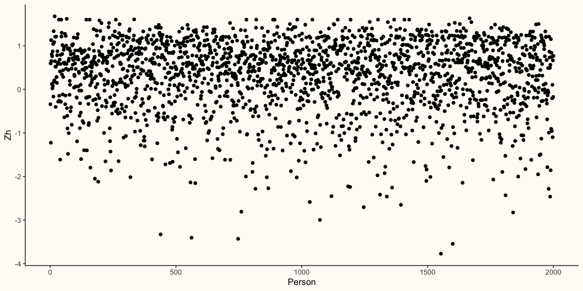
Person fit addresses the question: “Does a respondent’s response pattern match what the model predicts?”
There are different types of indices, but we will focus on one: \(Z_{h}\).
With \(Z_{h}\) we want to look our for values less than -2 or greater than 2.

Examining Person Fit

person_fit <- mirt::personfit(twopl_fit)
head(person_fit)

     outfit    z.outfit     infit    z.infit         Zh
1 1.0632275  0.31418408 1.0929672  0.4618278 -0.3414184
2 0.9388919 -0.07760082 0.7819367 -0.7185556  0.5961149
3 1.4219239  1.35352724 1.2869411  1.1084323 -1.2240626
4 0.6915336 -0.70417375 0.7933499 -1.2822548  1.1306864
5 0.7226860 -0.37995234 0.8674085 -0.5988320  0.6504189
6 0.8046861 -0.64577903 0.8615683 -0.8345722  0.8041080

Plotting Person Fit

Model Comparison

1PL \(\subset\) 2PL \(\subset\) 3PL \(\subset\) 4PL
We can use a log likelihood test to determine which model fits the data the best.

Estimating Theta

Using our estimated model, we can estimate (or predict) what an individual’s theta is. We can then use that prediction in other models as a predictor of some kind.
We can estimate theta using several different techniques. They should all produce fairly similar estimates:
- Maximum Likelihood Estimation
- Maximum a Posteriori (MAP - mode of posterior distribution)
- Expected a Posteriori (EAP - mean of posterior distribution)

Examining Theta Estimates

theta_mle <- mirt::fscores(twopl_fit, method = "ML", full.scores = TRUE, full.scores.SE = TRUE)
theta_map <- mirt::fscores(twopl_fit, method = "MAP", full.scores = TRUE, full.scores.SE = TRUE)
theta_eap <- mirt::fscores(twopl_fit, method = "EAP", full.scores = TRUE, full.scores.SE = TRUE)

# A tibble: 6 × 6
  THETA_MLE THETA_MLE_SE THETA_MAP THETA_MAP_SE THETA_EAP THETA_EAP_SE
      <dbl>        <dbl>     <dbl>        <dbl>     <dbl>        <dbl>
1    -0.274        0.489    -0.221        0.437    -0.238        0.447
2    -0.608        0.519    -0.482        0.452    -0.510        0.461
3    -0.408        0.500    -0.327        0.442    -0.349        0.452
4     0.910        0.520     0.722        0.448     0.749        0.458
5     1.36         0.582     1.03         0.472     1.07         0.482
6     0.294        0.477     0.239        0.430     0.244        0.440

Correlating Theta

          THETA_MLE THETA_MAP THETA_EAP
THETA_MLE     1.000     0.994     0.994
THETA_MAP     0.994     1.000     1.000
THETA_EAP     0.994     1.000     1.000

Estimating Item Parameters

Like CFA, there are different estimators available. We will talk about three:
- Joint Maximum Likelihood Estimation (Don’t use this!)
- Marginal Maximum Likelihood Estimation (Most defaults use this)
- Bayesian Estimation (Can be best of the three, but needs priors)

Readings for Next Week

Lang & Tay (2021)