Generalizability Theory
Overview
- Introduction to Generalizability Theory (GT)
- Example of a Generalizability and Decision Study
- Ideas about Advanced GT Topics
What is Generalizability Theory
- Generalizability theory is a framework that provides the theoretical and statistical tools needed to design and evaluate a measurement system (as opposed to a single measure). It takes a broader view of the dependability of measurements compared to Classical Test Theory (CTT).
Generalizability vs Reliability
Reliability asks how accurately observed score measures reflect their true score, whereas generalizability asks how accurately we can generalize a measurement to a universe of (predefined) situations.
The cost, however, is added complexity. GT comes with A LOT of theoretical and statistical complexity compared to CTT.
Designing a Measurement System
A measurement system is a set of interrelated elements that act together to produce a measurement. Unlike CTT, which largely focuses on designing a singular measure (i.e. scale), GT focuses on designing a measurement system with the following elements:
- Object of Measurement
- Measurement Facets (Sources of Error)
- Measurement Design
- Purpose of the Measurement
Example: Peformance Evaluation System
A small organization wants to work with you to develop a performance evaluation tool and give you free reign to design a study to evaluate its generalizability. You work with job incumbents and SMEs to develop an initial 10 item scale that measures an employee’s task performance. This tool is designed to be used by an evaluator to rate an employee’s performance. You get a sample of 100 employees and 10 evaluators to rate each employee.
Performance Evaluation Example: Data Frame
Object of Measurement
The object of measurement is the object in a measurement system that is being assigned scores (measurements). It is the object we are trying to differentiate among. In most behavioral and social science applications this will be persons.
Symmetry of Generalizability Theory states that any object (facet) in a measurement system can be the object of measurement (Cardinet et al., 1976). It is up to the researcher to determine this.
In our example, the object of measurement is the employee.
Sources of Error
- GT allows you to specify multiple sources of error, which are referred to as measurement facets, that lead to error in your measurement system.
- Common measurement facets: items, raters, occasions, forms
- Each measurement facet will generally have two or more conditions, which represent different replications (levels) of the facet.
Performance Evaluation: Measurement Facets
| 1 | 2 | 3 | 4 | 5 | 6 | 7 | 8 | 9 | 10 |
|---|---|---|---|---|---|---|---|---|---|
| 1000 | 1000 | 1000 | 1000 | 1000 | 1000 | 1000 | 1000 | 1000 | 1000 |
| 1 | 2 | 3 | 4 | 5 | 6 | 7 | 8 | 9 | 10 |
|---|---|---|---|---|---|---|---|---|---|
| 1000 | 1000 | 1000 | 1000 | 1000 | 1000 | 1000 | 1000 | 1000 | 1000 |
Random vs Fixed Facets
- Measurement facets can be considered fixed or random:
- Fixed Facet: The conditions of the measurement facet are exhaustive of all the conditions we wish to generalize across.
- Random Facet: The conditions of the measurement facet are a sample from a larger universe and are exchangeable with other samples from the universe.
- There are a lot of good reasons to treat all of our measurement facets as random–at least initially. In fact, internal consistency in CTT treats items as a random measurement facet.
Measurement Design
- The measurement design describes how the measurement facets and object of measurement are structured in relation to one another. There are two foundational structural features:
- Crossed Measurement Designs
- Nested Measurement Designs
Performance Evaluation: Measurement Design
, , RESP_ID = 1

        ITEM_ID
RATER_ID 1 2 3 4 5 6 7 8 9 10
      1  1 1 1 1 1 1 1 1 1  1
      2  1 1 1 1 1 1 1 1 1  1
      3  1 1 1 1 1 1 1 1 1  1
      4  1 1 1 1 1 1 1 1 1  1
      5  1 1 1 1 1 1 1 1 1  1
      6  1 1 1 1 1 1 1 1 1  1
      7  1 1 1 1 1 1 1 1 1  1
      8  1 1 1 1 1 1 1 1 1  1
      9  1 1 1 1 1 1 1 1 1  1
      10 1 1 1 1 1 1 1 1 1  1
, , RESP_ID = 2
ITEM_ID
RATER_ID 1 2 3 4 5 6 7 8 9 10
1 1 1 1 1 1 1 1 1 1 1
2 1 1 1 1 1 1 1 1 1 1
3 1 1 1 1 1 1 1 1 1 1
4 1 1 1 1 1 1 1 1 1 1
5 1 1 1 1 1 1 1 1 1 1
6 1 1 1 1 1 1 1 1 1 1
7 1 1 1 1 1 1 1 1 1 1
8 1 1 1 1 1 1 1 1 1 1
9 1 1 1 1 1 1 1 1 1 1
10 1 1 1 1 1 1 1 1 1 1Complex Measurement Designs
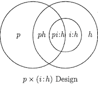
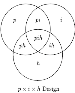
- Many different measurement designs can arise by combining crossed and nested designs together:
- Persons x Items: Persons crossed with Items
- Raters:Persons x Items: Raters nested within People crossed with Items
- Persons x Items:Forms: Persons crossed with Items nested within Alternate Forms
- Persons x Occasions x Items:Forms: Persons Crossed with Occasions crossed with Items nested within Forms
Statistical Model Underlying GT
\[\begin{align} X_{pir} & = \mu \;\; \text{(Grand Mean)}\\ & + \mu_{p}-\mu \;\; \text{(Person Effect)}\\ & + \mu_{i}-\mu \;\; \text{(Item Effect)}\\ & + \mu_{r}-\mu \;\; \text{(Rater Effect)}\\ & + \mu_{pi}-\mu_{p}-\mu{i}+\mu \;\; \text{(Person x Item Effect)}\\ & + \mu_{pr}-\mu_{p}-\mu{r}+\mu \;\; \text{(Person x Rater Effect)}\\ & + \mu_{ir}-\mu_{i}-\mu{r}+\mu \;\; \text{(Item x Rater Effect)}\\ & + X_{pir} - \mu_{pi} - \mu_{pr} - \mu_{ir} + \mu_{p} + \mu_{r} + \mu_{i} - \mu \;\; \text{(Residual)} \end{align}\]
Statistical Model Underlying GT
\[\begin{align} X_{pir} & = \mu \;\; \text{(Grand Mean)}\\ & + \nu_{p} \;\; \text{(Person Effect)}\\ & + \nu_{i} \;\; \text{(Item Effect)}\\ & + \nu_{r} \;\; \text{(Rater Effect)}\\ & + \nu_{pi} \;\; \text{(Person x Item Effect)}\\ & + \nu_{pr} \;\; \text{(Person x Rater Effect)}\\ & + \nu_{ir} \;\; \text{(Item x Rater Effect)}\\ & + e_{pir} \;\; \text{(Residual)} \end{align}\]
Variance Component Model
- At its statistical core, GT is a variance component model. GT decomposes the observed score variance into the sum of the object of measurement’s and the measurement facets’ variance components.
\[\sigma^2_{X_{pir}}=\sigma^2_{p}+\sigma^2_{i}+\sigma^2_{r}+\sigma^2_{pi}+\sigma^2_{pr}+\sigma^2_{ir}+\sigma^2_{e}\]
Variance Components
- Variance components are population parameters that describe the amount of variation for each of the random measurement facets and the object of measurement. Whereas CTT focused a lot on estimating reliability coefficients, GT is focused on estimating variance components:
- \(\sigma^2_{p}\): Amount of variation due to individuals’ differences
- \(\sigma^2_{r}\): Amount of variation among different raters (some raters are more lenient than others)
- \(\sigma^2_{pr}\): Amount of variation among different person x rater pairs
Visualizing Variance Components
Generalizability Study (G-Study)
A Generalizability Study is a study focused on designing a specific measurement system.
The main focus of a G-Study is to accurately estimate all of the variance components associated with the object of measurement and measurement facets. These estimates can then be used to inform future studies.
G-Studies are most informative when the measurement design is fully crossed and all the measurement facets are considered random as this allows one to estimate variance components that contribute to measurement error.
Populations and Universe of Admissible Observations
In a G-Study, objects of measurements are assumed to be drawn from a larger population and random measurement facets are assumed to be drawn from a universe of admissible observations (UAO).
The researcher defines the UAO by selecting the measurement facets that make up the G-Study and defining the admissible conditions of the measurement facet (e.g. only items that measure task performance).
Universe Score & Universe Score Variance
Each person (object of measurement) has a universe score which is defined as the expectation taken over the entire universe of admissible observations. We can estimate the universe score with the person mean, \(\mu_{p}\). This is similar to the true score in CTT.
Universe score variance, \(\sigma^2_{p}\), is the variance of universe scores over all people in the population. It is similar to true score variance and it describes the extent to which people vary because of differences in the attribute being measured.
Error: Relative & Absolute
GT also differs from CTT in another important way: it allows one to investigate the impacts of both relative error and absolute error .
Relative Error: Error that causes the rankings of individuals to differ across conditions within the same facet (e.g. receiving a high rating from one rater and a low rating from another). It is the sum of all of the variance components that involve an interaction with the object of measurement.
Absolute Error: Error that causes the object of measurement’s observed score to differ from its universe score. It is the sum of all of the variance components except the universe score variance component.
Performance Evaluation Example: Relative Error
\[\sigma^2_{rel}=\sigma^2_{pi}+\sigma^2_{pr}+\sigma^2_{e}\]
Perfromance Evaluation Example: Absolute Error
\[\sigma^2_{abs}=\sigma^2_{i}+\sigma^2_{r}+\sigma^2_{pi}+\sigma^2_{pr}+\sigma^2_{ir}+\sigma^2_{e}\]
Performance Evaluation Example: G Study
- Determine your population
- Determine your UAO
- If possible, keep your measurement design fully crossed and all of your facets random
- Estimate the variance components
Performance Evaluation Example: Data Frame
- Remember what our data looks like. It is in long format, which means that each row contains a unique combination of
RESP_ID,ITEM_ID, andRATER_ID.
Performance Evaluation Example: Results
- To analyze our data, we will use the
lmerfunction from thelme4package. Thelmerfunction estimates a mixed-effects regression model (multilevel models are a special case of mixed-effect models).
Performance Evaluation Example: Results
Linear mixed model fit by REML ['lmerMod']
Formula: RESPONSE ~ 1 + (1 | RESP_ID) + (1 | ITEM_ID) + (1 | RATER_ID) +
    (1 | RESP_ID:ITEM_ID) + (1 | RESP_ID:RATER_ID) + (1 | ITEM_ID:RATER_ID)
   Data: data_e2

REML criterion at convergence: 52262.2

Scaled residuals:
    Min      1Q  Median      3Q     Max
-3.7653 -0.6106  0.0001  0.6208  3.5007

Random effects:
 Groups           Name        Variance Std.Dev.
 RESP_ID:RATER_ID (Intercept) 18.998   4.359
 RESP_ID:ITEM_ID  (Intercept)  4.529   2.128
 ITEM_ID:RATER_ID (Intercept)  3.318   1.821
 RESP_ID          (Intercept) 16.370   4.046
 RATER_ID         (Intercept)  7.666   2.769
 ITEM_ID          (Intercept)  3.303   1.817
 Residual                      5.945   2.438
Number of obs: 10000, groups:
RESP_ID:RATER_ID, 1000; RESP_ID:ITEM_ID, 1000; ITEM_ID:RATER_ID, 100; RESP_ID, 100; RATER_ID, 10; ITEM_ID, 10

Fixed effects:
            Estimate Std. Error t value
(Intercept)    3.295      1.148    2.87
Performance Evaluation Example: Results
# A tibble: 7 × 3
  VAR_COMP_NAME    VAR_COMP VAR_COMP_PROP
  <chr>               <dbl>         <dbl>
1 RESP_ID:RATER_ID    19.0          0.316
2 RESP_ID             16.4          0.272
3 RATER_ID             7.67         0.127
4 Residual             5.94         0.099
5 RESP_ID:ITEM_ID      4.53         0.075
6 ITEM_ID:RATER_ID     3.32         0.055
7 ITEM_ID              3.30         0.055
Decision Study
- A decision study is a study that is focused using some measurement system to make a specific set of decisions (generalizations). Oftentimes, the G-Study and D-Study use the exact same data, but in theory the G-Study should be conducted using a separate set of data and that data should be used to inform how the D-Study is designed.
Conducting a Decision Study
- To conduct a D-Study, one must:
- Decide on the Universe of Generalization
- Use the G-Study variance components to simulate what happens to the relative and absolute error as the conditions of any measurement facet increase.
Universe of Generalization
The universe of generalization is defined by the researcher as the conditions of a measurement facet that one wishes to generalize across.
The universe of generalization is the D-Study equivalent of the UAO and in many cases will be equivalent to the UAO. However, researchers may decide to define the universe of generalization by making changes to the UAO:
- Fix a previously random measurement facet
- Turn a crossed aspect of the measurement design into a nested aspect
The Utility of a Decision Study
- D-Studies allow the researcher to simulate how the absolute and relative errors change (usually decrease) before actually conducting their study. Think of it as a way to optimize the measurement system for a specific decision (Marcoulides, 1993):
- Explore how error variance shrinks by increasing the number of conditions
- Explore how error variance shrinks, but the generalizations narrow by fixing a facet
- Explore how error variance changes, by choosing to nest rather than cross two facets
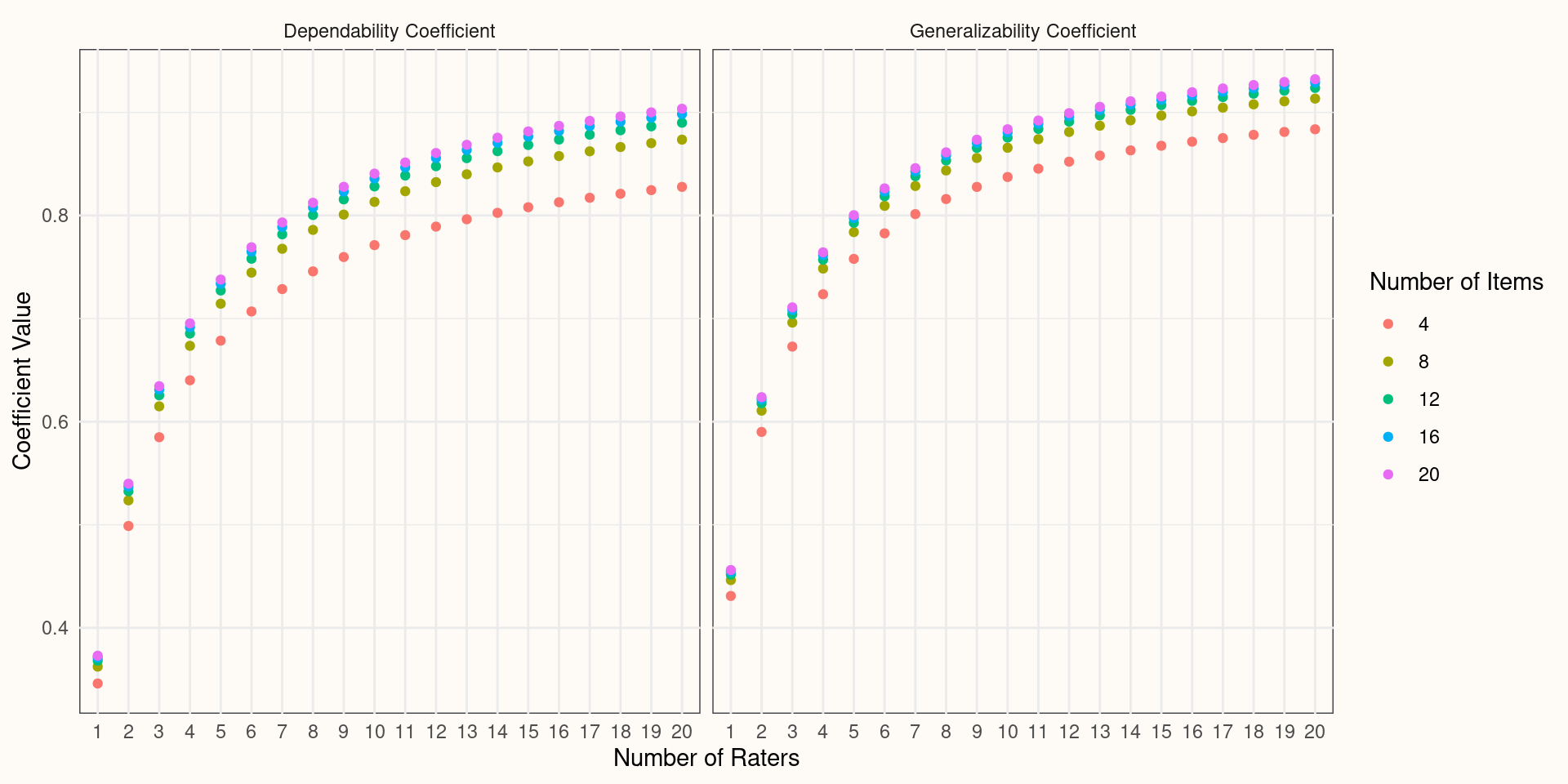
Reliability-Like Coefficients
- To gauge the impacts of each of those changes, we rely on two reliability-like coefficients: Generalizability Coefficient and Dependability Coefficient
\[\rho^2=\frac{\sigma^2_{p}}{\sigma^2_{p}+\frac{\sigma^2_{pi}}{n_{i}'}+\frac{\sigma^2_{pr}}{n_{r}'}+\frac{\sigma^2_{e}}{n_{i}'n_{r}'}}\]
\[\Phi=\frac{\sigma^2_{p}}{\sigma^2_{p}+\frac{\sigma^2_{i}}{n_{i}'} + \frac{\sigma^2_{r}}{n_{r}'}+\frac{\sigma^2_{pi}}{n_{i}'}+\frac{\sigma^2_{pr}}{n_{r}'}+\frac{\sigma^2_{e}}{n_{i}'n_{r}'}}\]
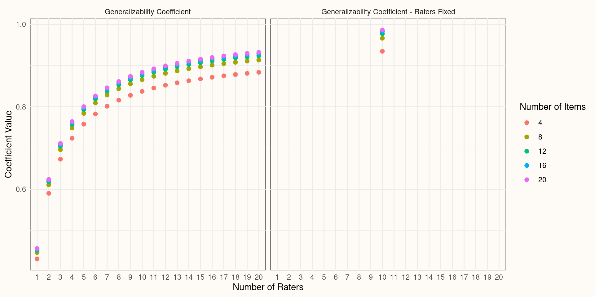
Performance Evaluation Example: Increasing Facet Conditions
Fixed Facets
Conceptually, a fixed facet is one where the sampled conditions exhaust the universe. That is, perhaps the 10 raters in our study are the only raters who will ever be providing ratings in this measurement system and thus we do not need to generalize to a larger universe of raters.
Mathematically, when we fix a facet, we are effectively averaging over it and redistributing its variance elsewhere.
This is GT’s explanation of the Reliability-Validity Paradox (Kane, 1982).
Redistributing Fixed Facet Variance
- If we fix raters in our D-Study, then:
\[\sigma^2_{p*}=\sigma^2_p + \frac{\sigma^2_{pr}}{n_r}\]
\[\sigma^2_{i*}=\sigma^2_i + \frac{\sigma^2_{ri}}{n_r}\]
\[\sigma^2_{e*}=\sigma^2_{pi}+\frac{\sigma^2_e}{n_r}\]
Performance Evaluation Example: Fixed Facets
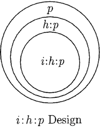
A Note on Nested Designs
- When one facet is nested within another facet it becomes impossible to separate the variance of the nested facet becomes confounded with the variance of the super-ordinate facet:
Why Nest a Facet in a D-Study?
If there are some kind of constraints for a facet, then there are instances where it makes sense to nest it. In our example, 10 raters each rating all 100 employees may not actually be feasible. It might make sense to nest raters within employees and have each rater rate 10 employees.
As a result, however, we could no longer estimate \(\sigma^2_{r}\) or \(\sigma^2_{pr}\) separate from one another.
Future Areas of Research
- Clarifying the assumptions of GT (they are murky at best)
- Expanding on Multivariate GT (yes we only just talked about univariate GT)
- See Jiang et al. (2020)
- Variance Component Estimation and Inference
- See LoPilato et al. (2015) or Jiang et al. (2022)
- Conditional GT Models using mixed-effect regression models
- See Putka et al. (2008)
- Exploring the effects and solutions to ill-structured measurement designs
- See Putka et al. (2008)
- Mixing economics, operations, and GT to optimize measurement systems
- See Marcoulides (1994)